Download
1 / 10
100 likes | 224 Vues
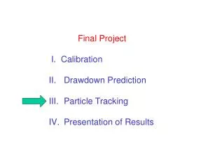
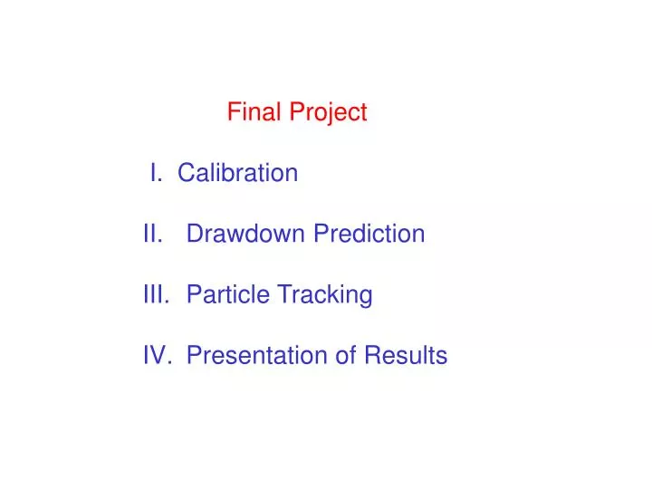
Final Project I. Calibration Drawdown Prediction Particle Tracking Presentation of Results. Schedule Week of April 14 : No lectures. Work on Parts I & II of Final Project April 22, 24: Particle tracking and Profile Models (PS6). Work on Part III of Final Project.

E N D
Final Project • I. Calibration • Drawdown Prediction • Particle Tracking • Presentation of Results
Schedule Week of April 14: No lectures. Work on Parts I & IIof Final Project April 22, 24: Particle tracking and Profile Models (PS6). Work on Part III of Final Project. April 24: 30 min in-class, closed book quiz. April 28, May 1: Group presentations of final project. May 6, May 8: Grid design/parameter selection & final thoughts. PS6 due on May 6.
Calibration Targets associated error calibration value 0.80 m 20.24 m Target with smaller associated error. Target with relatively large associated error.
Examples of Sources of Error • Surveying errors • Errors in measuring water levels • Interpolation error • Transient effects • Scaling effects • Unaccounted heterogeneities
Calibration parametersare uncertain parameters whose values are adjusted during model calibration. Typical calibration parameters include hydraulic conductivity and recharge rate.
Sensitivity analysis is used: • In automated calibration (inverse modeling) • (Sensitivity coefficients = • sum of squared residuals/parameter • or h/parameter) • As an uncertainty analysis after calibration
Automated calibration using inverse modeling Codes MODFLOWP – used in MODFLOW2000 GV Calibration PEST UCODE Available in GWV
Island Recharge Problem- Forward Problem L y 2L ocean Parameters known with certainty: R= 0.00305 ft/d K= 100 ft/day well Solve for head x ocean
Island Recharge Problem – Inverse Problem L y 2L ocean Head in well = 120 feet well Uncertain parameters R= 0.00305 ft/d K= 100 ft/day x ocean