Download
1 / 40
440 likes | 604 Vues
Topic 15: General Linear Tests and Extra Sum of Squares. Outline. Extra Sums of Squares with applications Partial correlations Standardized regression coefficients. General Linear Tests. Recall: A different way to look at the comparison of models Look at the difference

E N D
Outline • Extra Sums of Squares with applications • Partial correlations • Standardized regression coefficients
General Linear Tests • Recall: A different way to look at the comparison of models • Look at the difference • in SSE (reduce unexplained SS) • in SSM (increase explained SS) • Because SSM+SSE=SST, these two comparisons are equivalent
General Linear Tests • Models we compare are hierarchical in the sense that one (the full model) includes all of the explanatory variables of the other (the reduced model) • We can compare models with different explanatory variables such as • X1, X2 vs X1 • X1, X2, X3, X4, X5 vs X1, X2, X3 (Note first model includes all Xs of second)
General Linear Tests • We will get an F test that compares the two models • We are testing a null hypothesis that the regression coefficients for the extra variables are all zero • For X1, X2, X3, X4, X5 vs X1 , X2 , X3 • H0: β4 = β5 = 0 • H1: β4 and β5 are not both 0
General Linear Tests • Degrees of freedom for the F statistic are the number of extra variables and the dfE for the larger model • Suppose n=100 and we compare models with X1, X2, X3, X4, X5 vs X1 , X2 , X3 • Numerator df is 2 • Denominator df is n-6 = 94
Notation for Extra SS • SSE(X1,X2,X3,X4,X5) is the SSE for the fullmodel • SSE(X1,X2,X3) is the SSE for the reducedmodel • SSE(X4,X5 | X1,X2,X3) is the difference in the SSEs (reduced minus full) SSE(X1,X2,X3) - SSE(X1,X2,X3,X4,X5) • Recall can replace SSE with SSM
F test • Numerator : (SSE(X4,X5 | X1,X2,X3))/2 • Denominator : MSE(X1,X2,X3,X4,X5) • F ~ F(2, n-6) • Reject if the P-value ≤ 0.05 and conclude that either X4 or X5 or both contain additional information useful for predicting Y in a linear model that also includes X1, X2, and X3
Examples • Predict bone density using age, weight and height; does diet add any useful information? • Predict GPA using 3 HS grade variables; do SAT scores add any useful information? • Predict yield of an industrial process using temperature and pH; does the supplier of the raw material (categorical) add any useful information?
Extra SS Special Cases • Compare models that differ by one explanatory variable, F(1,n-p)=t2(n-p) • SAS’s individual parameter t-tests are equivalent to the general linear test based on SSM(Xi|X1,…, Xi-1, Xi+1 ,…, Xp-1)
Add one variable at a time • Consider 4 explanatory variables and the extra sum of squares • SSM (X1) • SSM (X2 | X1) • SSM (X3 |X1, X2) • SSM (X4 |X1, X2, X3) • SSM (X1) +SSM (X2 | X1) + SSM (X3 | X1, X2) + SSM (X4 | X1, X2, X3) =SSM(X1, X2, X3, X4)
One Variable added • Numerator df is 1 for each of these tests • F = (SSM / 1) / MSE( full ) ~ F(1, n-p) • This is the SAS Type I SS • We typically use Type II SS
KNNL Example p 257 • 20 healthy female subjects • Y is body fat • X1 is triceps skin fold thickness • X2 is thigh circumference • X3 is midarm circumference • Underwater weighing is the “gold standard” used to obtain Y
Input and data check options nocenter; data a1; infile ‘../data/ch07ta01.dat'; input skinfold thigh midarm fat; proc print data=a1; run;
Proc reg proc reg data=a1; model fat=skinfold thigh midarm; run;
Output Group of predictors helpful in predicting percent body fat
Output None of the individual t-tests are significant.
Summary • The P-value for F test is <.0001 • But the P-values for the individual regression coefficients are0.1699, 0.2849, and 0.1896 • None of these are below our standard significance level of 0.05 • What is the reason?
Look at this using extra SS proc reg data=a1; model fat=skinfold thigh midarm /ss1 ss2; run;
Output Notice how different these SS are for skinfold and thigh
Interpretation • Fact: the Type I and Type II SS are very different • If we reorder the variables in the model statement we will get • Different Type I SS • The same Type II SS • Could variables be explaining same SS and canceling each other out?
Run additional models • Rerun with skinfold as the explanatory variable proc reg data=a1; model fat=skinfold; run;
Output Skinfold by itself is a highly significant linear predictor
Use general linear test to see if other predictors contribute beyond skinfold proc reg data=a1; model fat= skinfold thigh midarm; thimid: test thigh, midarm; run;
Output Yes they are help after skinfold is in the model. Perhaps best model includes only two predictors
Use general linear test to assess midarm proc reg data=a1; model fat= skinfold thigh midarm; midarm: test midarm; run;
Output With skinfold and thigh in the model, midarm is not a significant predictor. This is just the t-test for this coef in full model
Other uses of general linear test • The test statement can be used to perform a significance test for any hypothesis involving a linear combination of the regression coefficients • Examples • H0: β4 = β5 • H0: β4 - 3β5 = 12
Partial correlations • Measures the strength of a linear relation between two variables taking into account other variables • Procedure to find partial correlation Xi , Y • Predict Y using other X’s • Predict Xi using other X’s • Find correlation between the two sets of residuals KNNL use the term coefficient of partial determination for the squared partial correlation
Pcorr2 option proc reg data=a1; model fat=skinfold thigh midarm / pcorr2; run;
Output Skinfold and midarm explain the most remaining variation when added last
Standardized Regression Model • Can help reduce round-off errors in calculations • Puts regression coefficients in common units • Units for the usual coefficients are units for Y divided by units for X
Standardized Regression Model • Standardized coefs can be obtained from the usual ones by multiplying by the ratio of the standard deviation of X to the standard deviation of Y • Interpretation is that a one sd increase in X corresponds to a ‘standardized beta’ increase in Y
Standardized Regression Model • Y = … + βX + … • = … + β(sX/sY)(sY/sX)X + … • = … + β(sX/sY)((sY/sX)X) + … • = … + β(sX/sY)(sY)(X/sX) + …
Standardized Regression Model • Standardize Y and all X’s (subtract mean and divide by standard deviation) • Then divide by n-1 • The regression coefficients for variables transformed in this way are the standardized regression coefficients
STB option proc reg data=a1; model fat=skinfold thigh midarm / stb; run;
Output Skinfold and thigh suggest largest standardized change
Reading • We went over 7.1 – 7.5 • We used program topic15.sas to generate the output