'Linear Hierarchical Models'

1. 'Linear Hierarchical Models' Definition Computation Applications ……the girlie way

2. Definition Hierarchical models provide a “framework” for both Classical inference (at first & second level) & Parametric Empirical Bayes (PEB) at first level (constrained by higher levels). Extension of the general linear model but with more variance components. Computation Both Classical and Bayesian approaches rest on estimating the covariance components Covariance components refer to the multiple variance components in the data (including within & between subject variance) Covariance components estimation is based on: Maximum Likelihood estimator (ML) or the Expectation Maximization (EM) algorithm = ML plus expectation step.

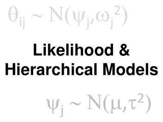
3. y = response variable; • X = design matrix/explanatory variables; • = parameters (betas) e = error 1st Level: Activation over scans (within session & subject) 2nd Level: Activation over sessions (within subjects) 3rd Level: Subject specific effects (over subjects) Parameters (q ): Quantities that determine the expected response (the effect) Can be estimated from mean without knowing its variance Hyperparameters: Variance of these quantities (within & between subject) (classically estimated using residual sum of squares)

4. Classical approach: how large are parameters with respect to standard error inference usually made at highest level (using between subject variability). Bayesian inference: probability of the parameters given the data prior covariance = error covariance at level above i.e. inference at lower levels (constrained by higher levels) e.g. Estimate of single subject can be constrained by knowledge of population using between subject variability from 2nd level as priors for parameters at first level. SPM uses activation over voxels (within subject) as the priors E.g. Within subject 1st Level: Activation over scans 2nd Level: Activation over voxels Both Classical and Bayesian approaches rest on estimating the covariance components

5. Covariance component estimation = estimating hyperparameters (within & between subject contributions to error) (hierarchically organised & linearly mixed variance components) Flattened to: Variance components are estimated with: Expectation Maximization (EM) Algorithm

6. ExpectationMaximization (EM) Algorithm EM estimates both parameters and hyperparameters from the data (using generic iterative / re-estimation procedure) E. step: finds expectation & covariance of the parameters holding hyperparameters fixed. M. step: updates maximum likelihood estimate of hyperparameters holding parameters fixed. EM used when hyperparameters of the likelihood and prior densities are not known. these hyperparameters become variance components that can be estimated using restricted maximum likelihood (ReML) ReML involves M step but not E step finds unknown variance components without explicit reference to the parameters. ……over to Raj