Download
1 / 70
860 likes | 1.71k Vues
Radio Propagation and Channel Modeling. Lecture 2 Outline. Review of Last Lecture Radio Propagation Characteristics Signal Propagation Overview Path Loss Models Free-space Path Loss Ray Tracing Models Simplified Path Loss Model Empirical Models Shadowing Combined Path Loss and Shadowing

E N D
Lecture 2 Outline • Review of Last Lecture • Radio Propagation Characteristics • Signal Propagation Overview • Path Loss Models • Free-space Path Loss • Ray Tracing Models • Simplified Path Loss Model • Empirical Models • Shadowing • Combined Path Loss and Shadowing • Multipath Channel Models • Channel modeling methods • MIMO Channel Models • Standardized channel models • An Example - WiNNER II Channel Model • Conclusions
Lecture 2 Outline • Review of Last Lecture • Radio Propagation Characteristics • Signal Propagation Overview • Path Loss Models • Free-space Path Loss • Ray Tracing Models • Simplified Path Loss Model • Empirical Models • Shadowing • Combined Path Loss and Shadowing • Multipath Channel Models • Channel modeling methods • MIMO Channel Models • Standardized channel models • An Example - WiNNER II Channel Model • Conclusions
Lecture 1 Review • Course Information • Wireless Vision • Technical Challenges • Multimedia Requirements • Current Wireless Systems • Spectrum Regulation and Standards
Lecture 2 Outline • Review of Last Lecture • Radio Propagation Characteristics • Signal Propagation Overview • Path Loss Models • Free-space Path Loss • Ray Tracing Models • Simplified Path Loss Model • Empirical Models • Shadowing • Combined Path Loss and Shadowing • Multipath Channel Models • Channel modeling methods • MIMO Channel Models • Standardized channel models • An Example - WiNNER II Channel Model • Conclusions
Slow Fast Very slow Propagation Characteristics • Path Loss (includes average shadowing) • Shadowing (due to obstructions) • Multipath Fading Pr/Pt Pt Pr v d=vt d=vt
Lecture 2 Outline • Review of Last Lecture • Radio Propagation Characteristics • Signal Propagation Overview • Path Loss Models • Free-space Path Loss • Ray Tracing Models • Simplified Path Loss Model • Empirical Models • Shadowing • Combined Path Loss and Shadowing • Multipath Channel Models • Channel modeling methods • MIMO Channel Models • Standardized channel models • An Example - WiNNER II Channel Model • Conclusions
Path Loss Modeling • Maxwell’s equations • Complex and impractical • Free space path loss model • Too simple • Ray tracing models • Requires site-specific information • Empirical Models • Don’t always generalize to other environments • Simplified power falloff models • Main characteristics: good for high-level analysis
d=vt Free Space (LOS) Model • Path loss for unobstructed LOS path • Power falls off : • Proportional to d2 • Proportional to l2(inversely proportional to f2) • More references: • Herry L. Bertoni, Radio Propagation for Modern Wireless Systems, Publishing House of Electronics Industry.
Ray Tracing Approximation • Represent wavefronts as simple particles • Geometry determines received signal from each signal component • Typically includes reflected rays, can also include scattered and defracted rays. • Requires site parameters • Geometry • Dielectric properties • Softwares:WiSE, SitePlanner, Planet EV, et.al.
Two Path Model • Path loss for one LOS path and 1 ground (or reflected) bounce • Ground bounce approximately cancels LOS path above critical distance • Power falls off • Proportional to d2(small d) • Proportional to d4(d>dc) • Independent of l (f)
General Ray Tracing • Models all signal components • Reflections • Scattering • Diffraction • Requires detailed geometry and dielectric properties of site • Similar to Maxwell, but easier math. • Computer packages often used
Simplified Path Loss Model • Used when path loss dominated by reflections. • Most important parameter is the path loss exponent g, determined empirically.
Empirical Models • Okumura model • Empirically based (site/freq specific) • Awkward (uses graphs) • Hata model • Analytical approximation to Okumura model • Cost 136 Model: • Extends Hata model to higher frequency (2 GHz) • Walfish/Bertoni: • Cost 136 extension to include diffraction from rooftops Commonly used in cellular system simulations
Main Points • Path loss models simplify Maxwell’s equations • Models vary in complexity and accuracy • Power falloff with distance is proportional to d2 in free space, d4 in two path model • General ray tracing computationally complex • Empirical models used in 2G simulations • Low accuracy (15-20 dB std) • Capture phenomena missing from formulas • Awkward to use in analysis • Main characteristics of path loss captured in simple model Pr=PtK[d0/d]g • Captures main characteristics of path loss
Lecture 2 Outline • Review of Last Lecture • Radio Propagation Characteristics • Signal Propagation Overview • Path Loss Models • Free-space Path Loss • Ray Tracing Models • Simplified Path Loss Model • Empirical Models • Shadowing • Combined Path Loss and Shadowing • Multipath Channel Models • Channel modeling methods • MIMO Channel Models • Standardized channel models • An Example - WiNNER II Channel Model • Conclusions
Shadowing • Models attenuation from obstructions • Random due to random # and type of obstructions • Typically follows a log-normal distribution • dB value of power is normally distributed • m=0 (mean captured in path loss), 4<s2<12 (empirical) • LLN used to explain this model • Decorrelated over decorrelation distance Xc Xc
Lecture 2 Outline • Review of Last Lecture • Radio Propagation Characteristics • Signal Propagation Overview • Path Loss Models • Free-space Path Loss • Ray Tracing Models • Simplified Path Loss Model • Empirical Models • Shadowing • Combined Path Loss and Shadowing • Multipath Channel Models • Channel modeling methods • MIMO Channel Models • Standardized channel models • An Example - WiNNER II Channel Model • Conclusions
Slow Combined Path Loss and Shadowing • Linear Model: y lognormal • dB Model 10logK Pr/Pt (dB) Very slow -10g log d
Outage Probability and Cell Coverage Area • Path loss: circular cells • Path loss+shadowing: amoeba cells • Tradeoff between coverage and interference • Outage probability • Probability received power below given minimum • Cell coverage area • % of cell locations at desired power • Increases as shadowing variance decreases • Large % indicates interference to other cells
K (dB) 2 sy 10g log(d0) Model Parameters from Empirical Measurements • Fit model to data • Path loss (K,g), d0 known: • “Best fit” line through dB data • K obtained from measurements at d0. • Exponent is MMSE estimate based on data • Captures mean due to shadowing • Shadowing variance • Variance of data relative to path loss model (straight line) with MMSE estimate for g Pr(dB) log(d)
Main Points • Random attenuation due to shadowing modeled as log-normal (empirical parameters) • Shadowing decorrelates over decorrelation distance • Combined path loss and shadowing leads to outage and amoeba-like cell shapes • Cellular coverage area dictates the percentage of locations within a cell that are not in outage • Path loss and shadowing parameters are obtained from empirical measurements
Lecture 2 Outline • Review of Last Lecture • Radio Propagation Characteristics • Signal Propagation Overview • Path Loss Models • Free-space Path Loss • Ray Tracing Models • Simplified Path Loss Model • Empirical Models • Shadowing • Combined Path Loss and Shadowing • Multipath Channel Models • Channel modeling methods • MIMO Channel Models • Standardized channel models • An Example - WiNNER II Channel Model • Conclusions
Statistical Multipath Model • Random # of multipath components, each with • Random amplitude • Random phase • Random Doppler shift • Random delay • Random components change with time • Leads to time-varying channel impulse response
Time Varying Impulse Response • Response of channel at t to impulse at t-t: • t is time when impulse response is observed • t-t is time when impulse put into the channel • t is how long ago impulse was put into the channel for the current observation • path delay for MP component currently observed
Received Signal Characteristics • Received signal consists of many multipath components • Amplitudes change slowly • Phases change rapidly • Constructive and destructive addition of signal components • Amplitude fading of received signal (both wideband and narrowband signals)
Narrowband Model • Assume delay spread maxm,n|tn(t)-tm(t)|<<1/B • Then u(t)u(t-t). • Received signal given by • No signal distortion (spreading in time) • Multipath affects complex scale factor in brackets. • Characterize scale factor by setting u(t)=d(t)
In-Phase and Quadrature components under CLT Approximation • In phase and quadrature signal components: • For N(t) large, rI(t) and rQ(t) jointly Gaussian (sum of large # of random vars). • Received signal characterized by its mean, autocorrelation, and cross correlation. • If jn(t) uniform, the in-phase/quad components are mean zero, indep., and stationary.
Auto and Cross Correlation • Assume fn~U[0,2p] • Recall that qn is the multipath arrival angle • Autocorrelation of inphase/quad signal is • Cross Correlation of inphase/quad signal is • Autocorrelation of received signal is
Uniform AOAs • Under uniform scattering, in phase and quad comps have no cross correlation and autocorrelation is • The PSD of received signal is Decorrelates over roughly half a wavelength Sr(f) Used to generate simulation values fc fc+fD fc-fD
Signal Envelope Distribution • CLT approx. leads to Rayleigh distribution (power is exponential) • When LOS component present, Ricean distribution is used • Measurements support Nakagami distribution in some environments • Similar to Ricean, but models “worse than Rayleigh” • Lends itself better to closed form BER expressions
Level crossing rate and Average Fade Duration • LCR: rate at which the signal crosses a fade value • AFD: How long a signal stays below target R/SNR • Derived from LCR • For Rayleigh fading • Depends on ratio of target to average level (r) • Inversely proportional to Doppler frequency t1 t2 t3 R
Markov Models for Fading • Model for fading dynamics • Simplifies performance analysis • Divides range of fading power into discrete regions Rj={g: Aj g < Aj+1} • Aj s and # of regions are functions of model • Transition probabilities (Lj is LCR at Aj): R2 A2 R1 A1 R0 A0
t t Wideband Channels • Individual multipath components resolvable • True when time difference between components exceeds signal bandwidth Narrowband Wideband
Scattering Function • Fourier transform of c(t,t) relative to t • Typically characterize its statistics, since c(t,t) is different in different environments • Underlying process WSS and Gaussian, so only characterize mean (0) and correlation • Autocorrelation is Ac(t1,t2,Dt)=Ac(t,Dt) • Statistical scattering function: r s(t,r)=FDt[Ac(t,Dt)] t
Multipath Intensity Profile • Defined as Ac(t,Dt=0)= Ac(t) • Determines average (TM ) and rms (st) delay spread • Approximate max delay of significant m.p. • Coherence bandwidth Bc=1/TM • Maximum frequency over which Ac(Df)=F[Ac(t)]>0 • Ac(Df)=0 implies signals separated in frequency by Df will be uncorrelated after passing through channel Ac(t) TM t Ac(f) f t Bc 0
Doppler Power Spectrum • Sc(r)=F[Ac(t=0,Dt)]= F[Ac(Dt)] • Doppler spread Bd is maximum doppler for which Sc (r)=>0. • Coherence time Tc=1/Bd • Maximum time over which Ac(Dt)>0 • Ac(Dt)=0 implies signals separated in time by Dt will be uncorrelated after passing through channel Sc(r) r Bd
Main Points • Statistical multipath model leads to a time-varying channel impulse response • Received signal has random amplitude fluctuations • Narrowband model and CLT lead to in-phase/quad components that are stationary Gaussian processes • Processes completely characterized by their mean, autocorrelation, and cross correlation. • Assuming uniform phase offsets, process is zero mean with joint expectation also zero.
Main Points • Narrowband model has in-phase and quad. comps that are zero-mean stationary Gaussian processes • Auto and cross correlation depends on AOAs of multipath • Uniform scattering makes autocorrelation of inphase and quad follow Bessel function • Signal components decorrelate over half wavelength • Cross correlation is zero (in-phase/quadratureindep.) • The power spectral density of the received signal has a bowel shape centered at carrier frequency • PSD useful in simulating fading channels
Main Points • Narrowband fading distribution depends on environment • Rayleigh, Ricean, and Nakagami all common • Average fade duration determines how long a user is in continuous outage (e.g. for coding design) • Markov model approximates fading dynamics. • Scattering function characterizes rms delay and Doppler spread. Key parameters for system design.
Main Points • Delay spread defines maximum delay of significant multipath components. Inverse is coherence bandwidth of channel • Doppler spread defines maximum nonzero doppler, its inverse is coherence time
Lecture 2 Outline • Review of Last Lecture • Radio Propagation Characteristics • Signal Propagation Overview • Path Loss Models • Free-space Path Loss • Ray Tracing Models • Simplified Path Loss Model • Empirical Models • Shadowing • Combined Path Loss and Shadowing • Multipath Channel Models • Channel modeling methods • MIMO Channel Models • Standardized channel models • An Example - WiNNER II Channel Model • Conclusions
Lecture 2 Outline • Review of Last Lecture • Radio Propagation Characteristics • Signal Propagation Overview • Path Loss Models • Free-space Path Loss • Ray Tracing Models • Simplified Path Loss Model • Empirical Models • Shadowing • Combined Path Loss and Shadowing • Multipath Channel Models • Channel modeling methods • MIMO Channel Models • Standardized channel models • An Example - WiNNER II Channel Model • Conclusions
Physical MIMO channel modeling • Multidimensional channel modeling • The double-directional channel impulse response • Multidimensional correlation functions and stationarity • Channel fading, K-factor and Doppler spectrum • Power delay and direction spectra • From double-direction propagation to MIMO channels • Statistical properties of the channel matrix • Discrete channel modeling : sampling theorem revisited • Physical versus analytical models • 1. C. Oestges and B. Clerckx, MIMO Wireless Communications: From Channel Models to Space-Time Code Design. Academic Press, 2007.
Physical MIMO channel modeling(cont) • Electromagnetic models • Ray-based deterministic methods • Multi-polarized channel • Geometry-based models • One-ring model • Two-ring model • Combined elliptical-ring model • Elliptical and circular models • Extension of geometry-based models to dual-polarized channels
Physical MIMO channel modeling(cont) • Empirical models • ExtendenSaleh-Valenzuela model • Stanford university interim channel models • COST models
Analytical MIMO channel models • General representations of correlated MIMO channels • Rayleigh fading channels • Ricean fading channels • Dual-polarized channels • Double-Rayleigh fading model for keyhole channels • Simplified representations of Guassian MIMO channels • The Kronecker model • Virtual channel representation • The eigenbeam model
Analytical MIMO channel models (cont) • Propagation-motivated MIMO metrics • Comparing models and correlation matrices • Characterizing the multipath richness • Measuring the non-stationarity of MIMO channels