Download
1 / 25
260 likes | 384 Vues
Correlating aftershock sequences properties to earthquake physics. J. Woessner S.Wiemer, S.Toda. Motivation. S1. S3. S2. Mc = 2.1 ± 0.18 b = 1.28 ± 0.16. S2. Mc = 1.5 ± 0.11 b = 0.73 ± 0.04. S3. S1. Stress tensor heterogeneity. b-value diversity. Hector Mine, 1999.

E N D
Correlating aftershock sequences properties to earthquake physics J. Woessner S.Wiemer, S.Toda
Motivation S1 S3 S2 Mc = 2.1±0.18 b = 1.28±0.16 S2 Mc = 1.5±0.11 b = 0.73 ± 0.04 S3 S1 Stress tensor heterogeneity b-value diversity Hector Mine, 1999 Big Bear, 1992 Landers, 1992 Wiemer et al. (2002)
Motivation Rotation of maximum principal stress axis (S1) MW=7.3, Landers, 1992 Background orientation : S1 N7°E Heterogeneous Emerson-Camp Rock ß > 45° Latitude [deg] Homestead valley Misfit angle ß [deg] Johnson valley S1 S2 S3 Homogeneous S1 Longitude [deg]
Aftershock activity – Local stress field • Relate b-values to stress field heterogeneity ß:H1: Stress tensor heterogeneity correlates positively with b-values • Investigate spatio-temporal behavior of the local stress field using aftershock focal mechanisms:H2: Stress tensor heterogeneity decreases with time
Aftershock activity – Local stress field • Evaluate Heterogeneous Post Seismic Stress Field Hypothesis (Michael et al., 1990) :H3: The rotation of the stress tensor axis correlates with regions of high slip and readjusts with time to the regional stress field • Introduce conceptual model
Study Regions and Data Sets SCSN:- Parametric earthquake catalogs from SCEDC- Fault Plane Solution catalog (FPS) NCSN:- Parametric earthquake catalogs from NCEDC- Fault Plane Solution catalog (FPS) Study Regions Data Sets • 1983 Coalinga • 1989 Loma Prieta • 1992 Landers • 1994 Northridge • 1999 Hector Mine
Method • Spatial and temporal analysis of the magnitude of completeness Mc (Woessner & Wiemer, 2005) • Spatial and temporal mapping ofb-values LogN = a – bM (M ≥ Mc) • Spatial and temporal mapping of stress tensor (Michael, 1984; Gephart, 1984):determination the stress tensor axis orientation and heterogeneity
Measures of Heterogeneity S1 S3 S2 ß Angular misfit ß: Angular misfit between the slip direction from the aftershock and the uniform stress tensor perfectly fitting the main shock FM (Michael, 1984, 1987, 1990) Summary:Measures are equivalent and scale linearly heterogeneous Stress tensor variance: Describes the fit of the observed focal mechanismto a homogeneous stress tensor. High variance => high heterogeneity of the stress field!
Stress tensor heterogeneity – b-value H1: Stress tensor heterogeneity correlates positively with b-values Is the heterogeneity related to the b-value distribution?
Landers: Magnitude of completeness Emerson – Camp Rock fault Northern part: Catalog complete for larger magnitudes Southern part: Catalog complete to small magnitudes Homesteadvalley fault Johnson valley fault
Stress tensor heterogeneity – b-value S2 S3 S1 MW=7.3, Landers, 1992 b = 0.73± 0.03 b = 1.13± 0.08
Stress tensor heterogeneity – b-value N S Homestead valley fault Emerson – Camp Rock fault Johnson valley fault Wald & Heaton (1994) Downdip distance [km] Slip [cm] b-value Misfit angle ß Along strike distance [km]
Stress tensor heterogeneity – b-value From Map From Cross-section Positive correlation: high b-values – high misfit angle! But only seen for Landers
Correlation for Other Events Coalinga 1983 Loma Prieta 1989 Hector Mine 1999 Coalinga: positive correlation Loma Prieta: ambiguous Hector Mine: ?
Temporal dependence of ß H2: Stress tensor heterogeneity decreases with time What is the temporal dependence of the stress tensor heterogeneity ß (and the rotation of S1)? How does it compare to the aftershock sequence duration?
Temporal dependence: Landers Emerson / Camp rock fault Pre-mainshock Time series Post-mainshock Prior to Landers Post Landers1975-1992 2 months ß=30°ß=78° Homogeneous! Heterogeneous!
Temporal dependence: Coalinga / Loma Prieta Coalinga, 1983 Loma Prieta, 1989
Aftershock sequence duration: Ta Landers: Emerson-Camp Rock Coalinga Ta 25.2–63.2y Ta 17.1–27.2y Loma Prieta Ta 8.8–11.7y
Summary • H1: Positive correlation of b and ß only for the Landers event • Probably not the fundamental relationDifferential stress (Schorlemmer et al., 2005) • H2: Stress tensor heterogeneity decreases with time • Seen for all events • Time-scale is smaller than aftershock sequence duration • Results support the HPSSF-hypothesis
Main shock slip – Stress field H3: The rotation of the stress tensor axis correlates with regions of high slip and readjusts with time to the regional stress field How are the stress field heterogeneity and the rotations of the maximum stress axis S1 related to main shock slip?
Main shock slip - Stress tensor heterogeneity Morgan Hill (1984) Parkfield (2004) Heaton & Hartzell (1988) C. Ji (2005) No heterogeneity observed!
Main shock slip - Stress tensor heterogeneity Loma Prieta (1989) Beroza (1991)
Main shock slip - Stress tensor heterogeneity Homestead valley fault Emerson – Camp Rock fault Johnson valley fault Downdip distance [km] Slip [cm] Misfit angle ß Along strike distance [km] Landers (1992) N S
Conceptual model Stress tensor inversion Coulomb stress transfer model S1 [East of North] Latitude [deg] Longitude [deg] S1 = without coseismic stress change (N7°E)S1 = with coseismic stress change
Conclusion & Outlook • Results support the HPSSF-hypothesis • Case studies show difference between small and large ruptures More quantification needed! Possibilities of conceptual model: • Constrain absolute size of regional background stress fieldHomogeneous with slight variations • Explain temporal rotation depending on loading process: viscoelastic relaxation?