Download
1 / 34
350 likes | 558 Vues
Interactive Geodesic Segmentation of n-Dimensional Medical Images on the Graphics Processor. A. Criminisi, T. Sharp and K. Siddiqui. State of the art v. our algorithm. State of the art segmentation algorithms QPBO Tree-reweighted mess. passing Random Walker Min-cut/max-flow

E N D
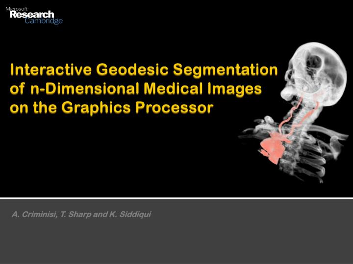
Interactive Geodesic Segmentation of n-Dimensional Medical Images on the Graphics Processor A. Criminisi, T. Sharp and K. Siddiqui
State of the art v. our algorithm • State of the art segmentation • algorithms • QPBO • Tree-reweighted mess. passing • Random Walker • Min-cut/max-flow • Belief propagation • Level Sets • Geodesic active contours • Region growing • K-means • Most based on complex energy minimization -> slow. • Properties of our algorithm • efficient on high-res./nD images • (~milliseconds) • easy to edit and fix • accurate • (e.g. handling of thin structures) • robust to noise • edge sensitive • captures uncertainty • (probabilistic output)
User interaction This is noisy! In order to obtain segmentation we need to encourage spatial smoothness Appearance likelihood is computed from histograms of intensities accumulated under the two brush strokes Input image User-entered brush strokes Likelihood of Fg v Bg Notation Legend • Green indicates high probability of Fg • Red indicates high probability of Bg • Grey for uncertain Output segmentation Point position Appearance likelihood Image intensities
A very efficient way of propagating image information around Background on geodesic distances
Geodesic distance Coronal CT view of r. kidney User-drawn brush stroke Binary mask of brush stroke Gradient and tangent vectors Image Binary mask Geodesic distance (Euclidean for =0) unit tangent vector Output geodesic distance D(p)
Geodesic distance transform: on the CPU, 2D Input Output geodesic distance GDT raster scan algorithm Forward pass: (top-left to bottom-right) with • Properties of algorithm • Contiguous memory access • Parallelizable • GPU-friendly • no region growing • no FMM • no level set Backward pass: (bottom-right to top-left) Image (8bpp) after W/L mapping!
Geodesic distance transform: on the GPU, 2D GPU algorithm implemented on NVidia processors using the CUDA language. Downward pass: In 2D four passes are necessary: top-bottom, bottom-top, left-right, right-left x 1 2 3 y Downward pass: with The downward pass. The red column shows pixels processed by the current thread. The distance values in the top (green) row Have already been computed. Distances along the arrow directions Are computed from texture reads as in the equation on the left panel. …similarly for the other three passes. Timings Typical CT image resolution = 512 X 512
Geodesic distance transform: on the GPU, 3D GPU algorithm implemented on NVidia processors using the CUDA language. Pass 1 of 6: In 3D six passes are necessary. Pass 1 of 6: 1 2 3 4 5 6 7 8 9 with direction of raster scan z x …similarly for the other five passes. y
How do we impose smoothness ? The Geodesic Symmetric Filter (GSF)
The GSF operator (I) Input binary mask M Signed distance Ds from boundary (in green) Signed distance Ds (zoomed) Signed distance from boundary with For ease of explanation we focus on a toy 2D example here.
The GSF operator (II) Geodesic morphology Geodesic dilation Dilated mask Geodesic erosion Signed distance Ds from boundary (green) Input binary mask M In each of the eroded and dilated masks part of the noise has been removed. Now we need to combine the two so as to remove all of the noise. Eroded mask
The GSF operator (III) Geodesic morphology, real example Geodesic erosion This is all extremely fast to compute. Distance Ds Geo. dilation , small d Geo. dilation , large d
The GSF operator (IV) Dilated mask Eroded mask Final, symmetric signed distance The new distance is much smoother than the original one because the effect of noise has been reduced. Symmetric signed distance Original signed distance
The GSF operator (V) Input binary mask M Symmetric signed distance Thresholding at 0 Final noise-free mask The GSF operator produces the final, noise-free mask Ms as: More examples with different noise patterns Distance Distance Input Filtered image Input Filtered image
The GSF operator on real-valued inputs GSF() Ms: output segmentation Real-valued case input GSF GGDT: Generalized Geodesic Distance Binary case was
Spatial smoothness for noise robustness smooth locked Ms: Output of GSF for small Ms: Output of GSF for large Larger values of produce smoother segmentations
The actual algorithm The Segmentation Algorithm
Output of GSF for fixed The actual segmentation algorithm (I) combine Appearance likelihood L a Distance term L d User brushes I. Compute pixel-wise likelihoods from user hints Data likelihood Appearance lik. with Distance term Soft input mask
Output of GSF for fixed The actual segmentation algorithm (II) GSF() Appearance likelihood La Distance signal Ld Output segmentation Ms II. Segmentation from pixel-wise likelihoods Geodesic symmetric distance Segmentation via GSF
Some segmentation results Aortic aneurism Three views of the segmented aorta. Bony structures (Bg) are shown faded to provide spatial context. Input is CT. The aorta, bottom of heart and pelvis have been segmented in 3D by our technique. The whole process (including user interaction) takes only a few seconds.
Some segmentation results Carotid arteries Three views of segmented carotids. Bony structures (Bg) are shown faded to provide spatial context. Input is CT. The carotids have been segmented interactively by our technique. Segmenting such long and thin structures is usually a problem for other existing algorithms.
Some segmentation results Studying the interaction between aorta and spine Three views of segmented aorta. The spine and heart (Bg) are shown faded to provide spatial context. Input is CT. The aorta and its thin bifurcations have been segmented by our technique in only a few seconds.
Some segmentation results A liver tumor Axial CT slice. The user segments a tumor in only a few milliseconds Automatic measurements of tumor The tumor has been segmented with a single user click. The whole operation has taken only a few milliseconds. Now that the tumor has been isolated statistics about its density, shape and texture are easily computed (right panel).
Some segmentation results Segmenting different structures in MR images
Some segmentation results Segmentation of noisy images Our segmentation Very noisy input image. Input is CT. Encouraging spatial smoothness is especially useful when dealing with very noisy images.
Some segmentation results Segmentation of noisy images Very noisy input image. Input is MR Our segmentation Encouraging spatial smoothness is especially useful when dealing with very noisy images.
Some segmentation results Testing accuracy in low-contrast images Very low-contrast input image Our segmentation The geodesic term in the definition of the geodesic distance enables segmentation in low contrast images.
Some segmentation results Capturing uncertainty in low-contrast regions Sharp segmentation (high confidence) because of strong gradients In low gradient regions the algorithm correctly returns low confidence segmentation
Accuracy: our algo. v min-cut [ Rother, C. Kolmogorov, V and Blake, A. GrabCut: Interactive foreground extraction using iterated graph cut. SIGGRAPH 2004. ] [Szeliski, R., Zabih, R., Scharstein, D., Veksler, O., Kolmogorov, V., Agarwala, A., Tappen, M., Rother, C.: A comparative study of energy minimization methods for markov random fields. In: ECCV. (2006)] Images and ground-truth from the standard GrabCut test dataset Not much of a difference in terms of accuracy.
Efficiency: our algo. v min-cut [ Rother, C. Kolmogorov, V and Blake, A. GrabCut: Interactive foreground extraction using iterated graph cut. SIGGRAPH 2004. ] • up to 60X speed up compared to min-cut. • with similar accuracy
Efficiency: our algo. v Bai et al. 2007 [ Bai, X. and Sapiro, G. A geodesic framework for fast interactive image and video segmentation and matting. ICCV 2007, Rio, Brasil. ] • up to 30X speed up compared to Bai et al., while avoiding topology issues. • also, Bai et al. do not impose spatial smoothness