Download
1 / 6
70 likes | 304 Vues
EOQ History. Interest on capital tied up in wages, material and overhead sets a maximum limit to the quantity of parts which can be profitably manufactured at one time; “set-up” costs on the job fix the minimum. Experience has shown one manager a way to determine the economical size of lots.

E N D
EOQ History • Interest on capital tied up in wages, material and overhead sets a maximum limit to the quantity of parts which can be profitably manufactured at one time; “set-up” costs on the job fix the minimum. Experience has shown one manager a way to determine the economical size of lots. • Early application of mathematical modeling to Scientific Management • Introduced in 1913 by Ford W. Harris, “How Many Parts to Make at Once”
MedEquip Example • Small manufacturer of medical diagnostic equipment. • Purchases standard steel “racks” into which components are mounted. • Metal working shop can produce (and sell) racks more cheaply if they are produced in batches due to wasted time setting up shop. • MedEquip doesn’t want to tie up too much precious capital in inventory. • Question: how many racks should MedEquip order at once?
EOQ Modeling Assumptions 1.Production is instantaneous – there is no capacity constraint and the entire lot is produced simultaneously. 2.Delivery is immediate – there is no time lag between production and availability to satisfy demand. 3.Demand is deterministic – there is no uncertainty about the quantity or timing of demand. 4.Demand is constant over time – in fact, it can be represented as a straight line, so that if annual demand is 365 units this translates into a daily demand of one unit. 5.A production run incurs a fixed setup cost – regardless of the size of the lot or the status of the factory, the setup cost is constant. 6.Products can be analyzed singly – either there is only a single product or conditions exist that ensure separability of products.
Notation D demand rate (units per year) c unit production cost, not counting setup or inventory costs (dollars per unit) A fixed or setup cost to place an order (dollars) h holding cost (dollars per year); if the holding cost is consists entirely of interest on money tied up in inventory, then h = ic where i is an annual interest rate. Q the unknown size of the order or lot size decision variable
Inventory vs Time in EOQ Model Q Inventory Q/D 2Q/D 3Q/D 4Q/D Time
MedEquip Example Costs • D = 1000 racks per year • c = $250 • A = $500 (estimated from supplier’s pricing) • h = (0.1)($250) + 10 = $35 per unit per year