Download
1 / 48
500 likes | 527 Vues
Inventory Management. REORDER QUANTITY METHODS AND EOQ. Reorder Quantity Methods. Inventory Management. Reorder Quantity is the quantity of items to be ordered so as to continue production without any interruptions in the future .

E N D
Inventory Management REORDER QUANTITY METHODS AND EOQ
Reorder Quantity Methods Inventory Management • Reorder Quantity is the quantity of items to be ordered so as to continue production without any interruptions in the future. • Some of the methods employed in the calculation of reorder quantity are described below:
Reorder Quantity Methods (Cont’d) Inventory Management • Fixed Quantity System • Open access bin system • Two-bin system
Fixed Quantity System Inventory Management • The reorder quantity is a fixed one. • Time for order varies. • When stock level drops to reorder level, then order is placed. • Calculated using EOQ formula. Reorder level quantity (ROL or reorder point)= safety stock + (usage rate +lead time)
Open access bin system Inventory Management • Bin is filled with items to maximum level. • Open bins are kept at places nearer to the production lines. • Operators use items without making a record. • Items are replenished at fixed time. • This system is used for nuts and bolts. • Eliminates unnecessary paper work and saves time.
Two-bin system Inventory Management • Two bins are kept having items at different level. • When first bin is exhausted, it indicates reorder. • Second bin is a reserve stock and used during lead-time period.
EOQEconomic Order Quantity Inventory Management • EOQ = mathematical device for arriving at the purchase quantity of an item that will minimize the cost. • total cost = holding costs + ordering costs
EOQ Inventory Management So…What does that mean? • Basically, EOQ system helps you identify the most economical way to replenish your inventory by showing you the best order quantity. • EOQ is the order size that"minimizes" Total Costs.
EOQ System Inventory Management • Behavior of Economic Order Quantity (EOQ) Systems • Determining Order Quantities • Determining Order Points
Behavior of EOQ Systems Inventory Management • As demand for the inventoried item occurs, the inventory level drops. • When the inventory level drops to a critical point, the order point, the ordering process is triggered. • The amount ordered each time an order is placed is fixed or constant.
Behavior of EOQ Systems Inventory Management • When the ordered quantity is received, the inventory level increases. • An application of this type system is the two-bin system. • A perpetual inventory accounting system is usually associated with this type of system.
Determining Order Quantities Inventory Management • Basic EOQ • EOQ for Production Lots • EOQ with Quantity Discounts
Model I: Basic EOQ Inventory Management Typical assumptions made • Only one product is involved. • Annual demand requirements known. • Demand is even throughout the year. • Lead time does not vary. • Each order is received in a single delivery. • There are no quantity discounts.
Assumptions Inventory Management • Annual demand (D), carrying cost (C) and ordering cost (S) can be estimated. • Average inventory level is the fixed order quantity (Q) divided by 2 which implies • no safety stock • orders are received all at once
Assumptions Inventory Management • demand occurs at a uniform rate • no inventory when an order arrives • stock-out, customer responsiveness, and other costs are inconsequential. • acquisition cost is fixed, i.e., no quantity discounts
Assumptions Inventory Management • Annual carrying cost = (average inventory level) x (carrying cost) = (Q/2)C • Annual ordering cost = (average number of orders per year) x (ordering cost) = (D/Q)S
Definition of EOQ Components Inventory Management H = annual holding cost for one unit of inventory S = cost of placing an order, regardless of size P = price per unit d = demand per period D = annual demand L = lead time Q = Order quantity (this is what we are solving for)
Annual carrying cost Annual ordering cost Total cost = + Q D S H TC = + 2 Q Total Cost Inventory Management
EOQ Equation Inventory Management • Total annual stocking cost (TSC) = annual carrying cost + annual ordering cost = (Q/2)C + (D/Q)S • The order quantity where the TSC is at a minimum (EOQ) can be found using calculus (take the first derivative, set it equal to zero and solve for Q)
How does it work? Inventory Management • Total annual holding cost = (Q/2)H • Total annual ordering cost = (D/Q)S • EOQ: • Set (Q/2)H = (D/Q)S and solve for Q
Solve for Q algebraically Inventory Management • (Q/2)H = (D/Q)S • Q2 = 2DS/H • Q = square root of (2DS/H) = EOQ
Cost Minimization Goal Inventory Management The Total-Cost Curve is U-Shaped Holding Costs Annual Cost Ordering Costs (optimal order quantity) Order Quantity (Q)
Minimum Total Cost Inventory Management The total cost curve reaches its minimum where the carrying and ordering costs are equal. The Total-Cost Curve is U-Shaped Holding Costs Annual Cost Ordering Costs (optimal order quantity) Order Quantity (Q)
Example: Basic EOQ Inventory Management • Z-Company produces fertilizer to sell to wholesalers. One raw material: calcium nitrate is purchased from a nearby supplier at $22.50 per ton. Z-Company estimates it will need 5,750,000 tons of calcium nitrate next year. • The annual carrying cost for this material is 40% of the acquisition cost, and the ordering cost is $595.
Example: Basic EOQ Inventory Management • What is the most economical order quantity? • How many orders will be placed per year? c) How much time will elapse between orders?
Remember Inventory Management H = annual holding cost for one unit of inventory S = cost of placing an order, regardless of size P = price per unit d = demand per period D = annual demand L = lead time Q = Order quantity (this is what we are solving for)
Example: Basic EOQ Inventory Management • Economical Order Quantity (EOQ) D = 5,750,000 tons/year C = .40(22.50) = $9.00/ton/year S = $595/order Q = 27,573.135 tons per order
Example: Basic EOQ Inventory Management • Total Annual Stocking Cost (TSC) TSC = (Q/2)C + (D/Q)S = (27,573.135/2)(9.00) + (5,750,000/27,573.135)(595) = 124,079.11 + 124,079.11 = $248,158.22 Note: Total Carrying Cost equals Total Ordering Cost
Example: Basic EOQ Inventory Management • Number of Orders Per Year • = D/Q • = 5,750,000/27,573.135 • = 208.5 orders/year • Time Between Orders • = Q/D • = 1/208.5 • = .004796 years/order • = .004796(365 days/year) = 1.75 days/order Note: This is the inverse of the formula above.
Assignment The I-75 Carpet Discount Store in North Georgia stocks carpet in its warehouse and sells it through an adjoining showroom. The store keeps several brands and styles of carpet in stock; however, its biggest seller is Super Shag carpet. The store wants to determine the optimal order size and total inventory cost for this brand of carpet given an estimated annual demand of 10,000 yards of carpet, an annual carrying cost of $0.75 per yard, and an ordering cost of $150. The store would also like to know the number of orders that will be made annually and the time between orders (i.e., the order cycle) given that the store is open every day except Sunday, Thanksgiving Day, and Christmas Day (which is not on a Sunday). http://www.prenhall.com/divisions/bp/app/russellcd/PROTECT/CHAPTERS/CHAP12/HEAD03.HTM
Model II: EOQ for Production Lots Inventory Management • Used to determine the order size, production lot. • Differs from Model I because orders are assumed to be supplied or produced at a uniform rate (p) rather than the order being received all at once.
Model II: EOQ for Production Lots Inventory Management • It is also assumed that the supply rate, p, is greater than the demand rate, d • The change in maximum inventory level requires modification of the TSC equation • TSC = (Q/2)[(p-d)/p]C + (D/Q)S • The optimization results in
Example: EOQ for Production Lots Inventory Management • Electric Company buys coal from Coal Company to generate electricity. The seller company can supply coal at the rate of 3,500 tons per day for $10.50 per ton. The buyer company uses the coal at a rate of 800 tons per day and operates 365 days per year.
Example: EOQ for Production Lots Inventory Management • The buyer company’s annual carrying cost for coal is 20% of the acquisition cost, and the ordering cost is $5,000. • What is the economical production lot size? b) What is The buyer company ’s maximum inventory level for coal?
Example: EOQ for Production Lots Inventory Management Economical Production Lot Size D(demand)= 800 tons/day; D = 365(800)=292,000tons/year P(supply) = 3,500 tons/day for $10.50 per ton S(ordering cost)=$5,000/order.; C(carrying cost)=0.20(10.50)=$2.10/ton/year = 42,455.5 tons per order
Example: EOQ for Production Lots Inventory Management • Total Annual Stocking Cost (TSC) TSC = (Q/2)((p-d)/p)C + (D/Q)S = (42,455.5/2)((3,500-800)/3,500)(2.10) + (292,000/42,455.5)(5,000) = 34,388.95 + 34,388.95 = $68,777.90 Note: Total Carrying Cost equals Total Ordering Cost
Assignment Assume that the I-75 Outlet Store has its own manufacturing facility in which it produces Super Shag carpet. The ordering cost, Co, is the cost of setting up the production process to make Super Shag carpet. Recall Cc = $0.75 per yard and D = 10,000 yards per year. The manufacturing facility operates the same days the store is open (i.e., 311 days) and produces 150 yards of the carpet per day. Determine the optimal order size, total inventory cost, the length of time to receive an order, the number of orders per year, and the maximum inventory level. http://www.prenhall.com/divisions/bp/app/russellcd/PROTECT/CHAPTERS/CHAP12/HEAD03.HTM http://www.prenhall.com/divisions/bp/app/russellcd/PROTECT/CHAPTERS/CHAP12/HEAD03.HTM
Model III: EOQ with Quantity Discounts Inventory Management • Lower unit price on larger quantities ordered. • This is presented as a price or discount schedule, i.e., a certain unit price over a certain order quantity range • This model differs from Model I because the acquisition cost (ac) may vary with the quantity ordered, i.e., it is not necessarily constant.
Model III: EOQ with Quantity Discounts Inventory Management • Under this condition, acquisition cost becomes an incremental cost and must be considered in the determination of the EOQ • The total annual material costs (TMC) = Total annual stocking costs (TSC) + annual acquisition cost TSC = (Q/2)C + (D/Q)S + (D)ac
Model III: EOQ with Quantity Discounts Inventory Management To find the EOQ, the following procedure is used: 1. Compute the EOQ using the lowest acquisition cost. • If the resulting EOQ is feasible (the quantity can be purchased at the acquisition cost used), this quantity is optimal and you are finished. • If the resulting EOQ is not feasible, go to Step 2 2. Identify the next higher acquisition cost.
Model III: EOQ with Quantity Discounts Inventory Management 3.Compute the EOQ using the acquisition cost from Step 2. • If the resulting EOQ is feasible, go to Step 4. • Otherwise, go to Step 2. 4. Compute the TMC for the feasible EOQ (just found in Step 3) and its corresponding acquisition cost. 5. Compute the TMC for each of the lower acquisition costs using the minimum allowed order quantity for each cost. 6. The quantity with the lowest TMC is optimal.
Example: EOQ with Quantity Discounts Inventory Management A-1 Auto Parts has a regional tyre warehouse in Atlanta. One popular tyre, the XRX75, has estimated demand of 25,000 next year. It costs A-1 $100 to place an order for the tyres, and the annual carrying cost is 30% of the acquisition cost. The supplier quotes these prices for the tire: Q ac 1 – 499 $21.60 500 – 999 20.95 1,000 + 20.90
Example: EOQ with Quantity Discounts Inventory Management • Economical Order Quantity This quantity is not feasible, so try ac = $20.95 This quantity is feasible, so there is no reason to try ac = $21.60
Example: EOQ with Quantity Discounts Inventory Management • Compare Total Annual Material Costs (TMCs) TMC = (Q/2)C + (D/Q)S + (D)ac Compute TMC for Q = 891.93 and ac = $20.95 TMC2 = (891.93/2)(.3)(20.95) + (25,000/891.93)100 + (25,000)20.95 = 2,802.89 + 2,802.91 + 523,750 = $529,355.80
Example: EOQ with Quantity Discounts Inventory Management Compute TMC for Q = 1,000 and ac = $20.90 TMC3 = (1,000/2)(.3)(20.90) +(25,000/1,000)100 + (25,000)20.90 = 3,135.00 + 2,500.00 + 522,500 = $528,135.00 (lower than TMC2) The EOQ is 1,000 tyres at an acquisition cost of $20.90.
When to Reorder with EOQ Ordering Inventory Management • Reorder Point- When the quantity on hand of an item drops to this amount, the item is reordered. • Safety Stock- Stock that is held in excess of expected demand due to variable demand rate and/or lead time. • Service Level- Probability that demand will not exceed supply during lead time.
Determinants of the Reorder Point Inventory Management • The rate of demand • The lead time • Demand and/or lead time variability • Stock-out risk (safety stock)
Quantity Maximum probable demand during lead time Expected demand during lead time ROP Safety stock Time LT Safety Stock Inventory Management Safety stock reduces risk of Stock-out during lead time