Download
1 / 21
230 likes | 443 Vues
EOQ. Answers the Question “How Much to Order?” Assumptions : Instantaneous production Immediate delivery Deterministic demand Constant demand: D units/year Constant setup cost: A $/setup Independent products. EOQ view of Inventory. Order Quantity Q. Inventory. Time. Costs.

E N D
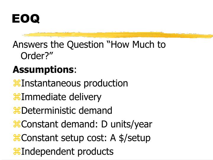
EOQ Answers the Question “How Much to Order?” Assumptions: • Instantaneous production • Immediate delivery • Deterministic demand • Constant demand: D units/year • Constant setup cost: A $/setup • Independent products
EOQ view of Inventory Order Quantity Q Inventory Time
Costs • Setup Costs • A $/setup • How many setups if we make Q each time? • Why not just make D units in one setup?
Inventory Cost • Usually billed as a “holding cost” • Essentially interest on the money tied up in inventory • h $/unit/year • Example: Holding 100 units for 6 months costs: ? • Inventory holding Cost • h*Average Inventory
A Model Lot Size or Order Quantity: Q units Average Inventory Level: Q/2units Annual Demand: D units/year Order Frequency: every D/Q times per year Average Variable Cost/Year: TVC = h*Q/2 +A*D/Q
The EOQ • Use Calculus to find the value of Q that minimizes TVC(Q) • Or...
The Economic Order Quantity h Q/2 = A D/Q Q2 = 2 A D/h Q = SQRT(2 A D/h) CAVEAT: Make sure you use commensurate units!
An Example • Raw Material X • Quarterly demand: 6,000 units • Cost per unit: ~ $25/unit • Holding Cost: say 10% per year • Transaction Cost: $100/order EOQ = SQRT(2 CT D/ CI) = SQRT(2 * 100 * 6,000/(0.025*25)) ~ 1,385 units per shipment
EPQ Answers the Question “How Much to Produce?” Assumptions: • Instantaneous production • Constant production rate: P > D units/year • Immediate delivery • Deterministic demand • Constant demand: D units/year • Constant setup cost: A$/setup • Independent products
EPQ view of Inventory Inventory Production Quantity Q Max Inv. Level Length of Prod. Run Time
A Model Lot Size or Production Quantity: Q units Average Inventory Level • Production run lasts: Q/P • Inventory grows at rate: (P-Q) • So, max inventory is: (P-D)Q/P = (1-D/P)Q • Average inventory is: (1-D/P)Q/2 Order Frequency: every D/Q times per year Average Variable Cost/Year: TVC = h*(1-D/P)Q/2 +A*D/Q
The EPQ • Use Calculus to find the value of Q that minimizes TVC(Q) • Or use the previous answer... • TVC = h*(1-D/P)Q/2 +A*D/Q = h’Q/2 +A*D/Q So, Q = SQRT(2 A D/h’) = SQRT(2AD/h(1-D/P))
An Example • Raw Material X • Quarterly demand: 6,000 units • Cost per unit: ~ $25/unit • Holding Cost: say 10% per year • Transaction Cost: $100/order • Quarterly Production Rate: 8,000 units EOQ = SQRT(2 CT D/ CI) = SQRT(2*100*6,000/(0.025*25*(1-6/8))) ~ 2,771 units per run
A Model • Divide the planning horizon into time buckets t = 1, 2, ..., T • Dt = units of demand in period t • ct = unit production cost in period t • At = setup cost in period t • ht = inventory holding cost in period t • Qt = the lot size in period t • It = units in inventory at the end of period t
Heuristics • Lot-for-lot: Make what is required each period. • Fixed Order Quantity: Order the EOQ • Period Order Quantity: Calculate the EOQ, Q. Convert to order frequency: T = Q/D. Orders sized to last for time T.