Download
1 / 24
240 likes | 351 Vues
Evidence for short correlation lengths of the noon-time equatorial electrojet – inferred from a comparison of satellite and ground magnetic data. C. Manoj National Geophysical Research Institute, Hyderabad, India. H. Lühr GeoForschungsZentrum – Potsdam, Germany S. Maus

E N D
Evidence for short correlation lengths of the noon-time equatorial electrojet – inferred from a comparison of satellite and ground magnetic data. C. Manoj National Geophysical Research Institute, Hyderabad, India. H. Lühr GeoForschungsZentrum – Potsdam, Germany S. Maus CIRES, University of Colorado, USA N. Nagarajan National Geophysical Research Institute , Hyderabad, India.
Equatorial Electrojet - generation Solar tidal effects causes current flow in the day time ionosphere E region (Sq) Sq current system sustains an eastward directed electrified from dawn-dusk at low latitude. A Hall current is then generated, carried by the upward moving electrons. The non-conductive boundaries above and below the lower ionosphere causes large vertical electric field build up. This vertical electric field (about 5 to 10 times stronger than the eastward electric field that produced it. This vertical field generates an eastward current called equatorial electrojet (EEJ) in noon-time ionosphere (Figure from Anderson et al, 2002)
Equatorial Electrojet – magnetic fields The equatorial electrojet produces strong enhancement of horizontal magnetic intensity within ±3° of the magnetic equator. EEJ has been studied using magnetometer array, rockets, radar, satellites… etc. etc.. Simulated horizontal magnetic anomaly at ground due to ionospheric currents (from CM4). Unit - nT
Equatorial Electrojet – magnetic fields A unique way of studying the EEJ is by using the differences in horizontal magnetic variations at an equatorial observatory from another observatory separated by 10°-15° in latitude. EEJ was also studied by satellite missions like POGO, Magsat, Oersted and CHAMP. LEO satellites, which flies above the ionosphere senses EEJ as negative signal at dip equator. Lühr et al, 2004
Some open questions on EEJ Lühr et al, 2004 reports uncorrelated current strength between successive CHAMP passes over EEJ. These passes are separated in space by ~23º and in time by ~93 minutes.
° 90 N ° 45 N ° ° ° ° ° ° ° ° ° ° 0 180 W 135 W 90 W 45 W 0 45 E 90 E 135 E 180 E ° 45 S ° 90 S -40 -30 -20 -10 0 10 20 30 40 ° 90 N ° 45 N ° ° ° ° ° ° ° ° ° ° 0 180 W 135 W 90 W 45 W 0 45 E 90 E 135 E 180 E ° 45 S ° 90 S Some open questions on EEJ UT 6 Is the observed variability in EEJ current strength due to spatial (23º) or temporal (93 minutes) effects ? 23º West and 93 minutes later UT 7:30
Some open questions on EEJ Are Sq and EEJ current systems coupled ? EEJ is often modeled as an equatorial enhancement of a coherent, large scale Sq current system (for eg. MacDaugall, 1979, CM4, Sabaka et al, 2004 ). Forbes (1981) concludes that EEJ and Sq are coupled current systems. This finding is also supported by Hesse (1982). However studies by Mann & Schlapp (1988) and Okeke (2006) shows poor correlation of horizontal magnetic fields between observatories within the equatorial region and outside of it. Also studies by Raghavarao & Anandarao (1987) finds that Sq and EEJ are decoupled.
How do we go about it ? While, from the ground, a continuous record of the current-induced magnetic field is obtained, polar orbiting satellites take just a snapshot of the latitudinal current distribution while passing over the equatorial region. The temporal variations recorded by a ground station can either be caused by a change in current strength or by a displacement of the current axis. Satellite measurements on the other hand give no information on the temporal variation of the EEJ but a good picture of the current geometry. By combining both data sets the advantages can be used to eliminate several ambiguities and answer the questions we discussed.
Roadmap Observatory and satellite data. Data processing Correlation analysis Results
Observatory data Distribution of the geomagnetic observatories used for the study. Hourly means of the horizontal intensities from 13 observatories. Period: Sep 2000 – Dec. 2002 Screened for Kp ≤ 2 to limit the analysis to magnetically quiet days.
0 100 10 UT (Hours) 0 20 -100 2000 2001 2002 2003 Time (Years) EEJ signals from ground data ΔHEEJ – ΔHNon-EEJ ΔH is the variation from midnight level. Average daily variation of the horizontal components of geomagnetic field observed at ETT with respect to the station HYB. Typically, the EEJ signal reaches up to 53 nT. The solid line represents a polynomial fit to the data. EEJ signals for 2000-2002
R L Satellite data Scalar magnetic field data from 2000 to 2002 Local Time : 10 to 13 Kp index ≤ 2 Total 1653 crossings Data reduction Main field (Pomme 1.4, Maus et al, 2005) Lithospheric field (MF2, Maus et al, 2002) Diamagnetic effect (Lühr et al, 2003) Large-scale magnetospheric fields by polynomial fitting Current density distribution was modeled by series of EW oriented current lines separated by 0.5º in latitude and located at an altitude of 108 km. Induction effect conductosphere at depth of 200 km Re-drawn from Lühr et al, 2004
Magnetic profile from CHAMP Predicted ground magnetic field profile due to the noon time equatorial electrojet from the CHAMP average current profile. The locations of geomagnetic observatories are plotted with respect to the dip-equator along the magnetic field profile
LT correction Since the satellite crosses the dip-equator at a certain LT and the corresponding observatory data may have a different LT, a correction needs to be applied to make the data set comparable. A degree-9 polynomial was used to find The ratio of expected EEJ strength at observatory and satellite local time
Sq correction By subtracting the data from non – equatorial observatory, we remove a part of the Sq variation at the equatorial observatory. The unresolved part corresponds to the latitudinal slope of the Sq between the observatory pair. Although none of the two stations is directly below the EEJ a daily variation of more than 50 nT is seen here. CM4 model (Sabaka et al, 2004) was used to obtain an estimate of the latitudinal slope of the Sq signal between the observatory pairs.
-30 -20 -10 100 100 100 CC 0.15 CC 0.49 CC 0.83 80 80 80 60 60 60 H D 40 40 40 20 20 20 0 0 0 0 0.1 0.2 0.3 0.4 0 0.1 0.2 0.3 0.4 0 0.1 0.2 0.3 0.4 0 10 20 100 100 100 CC 0.94 CC 0.81 CC 0.56 D H = 299.6 * I + -9.75 80 80 80 60 60 60 H D 40 40 40 20 20 20 0 0 0 0 0.1 0.2 0.3 0.4 0 0.1 0.2 0.3 0.4 0 0.1 0.2 0.3 0.4 A/m A/m A/m Correlation Analysis 1 0.5 Correlation Coefficient With LT correction 0 Without LT correction -0.5 -40 -30 -20 -10 0 10 20 30 40 Distance from Observatory in Degrees
Correlation Analysis Correlation coefficients as function of distance from the observatories. The central bin gives a high correlation between the satellite and ground data. However, the correlation decays very fast, when the satellite passes further away from the station longitude. Statistically significant correlation lengths of ~± 15º is observed in Indian and American sectors. Without Sq correction With Sq correction
Low correlation Is the observed variability in EEJ current strength due to spatial (23º) or temporal (93 minutes) effects ? From our ground/satellite comparison performed at various longitude separations we may conclude that this is primarily a spatial effect Reason ? The driving electric fields has large spatial scales (~ 30º) Since we have excluded the electric field, the conductivity may be responsible for the short-range coherence of the EEJ. A promising candidate for local conductivity modulation is plasma instability within the Cowling channel. Implications ?
1 0.8 0.6 Correlation coefficient 0.4 0.2 PND-HYB ETT-PND 0 -40 -20 0 20 40 Distance from the observatory in degrees 1 0.8 0.6 Correlation coefficient 0.4 ETT-PND 0.2 PND-HYB 0 -40 -20 0 20 40 Distance from observatory in degrees Sq and EEJ Without Sq correction ° 20 N Bombay Pune Hyderabad HYB ° 15 N Bangalore Madras PND ° 10 N Madurai ETT SRI LANKA Colombo ° With Sq correction 5 N ° ° 70 E ° ° E 90 ° 85 E 75 E 80 E
MOROCCO ° 30 N GUI ° 25 N WESTERN SAHARA 1 ° 20 N 0.8 MAURITANIA 0.6 Nouakchott 0.4 0.2 ° 15 N MBO 0 -0.2 Bamako -40 -20 0 20 40 GUINEA ° 10 N ° ° 20 W ° ° W 5 10 W 15 W Sq and EEJ Distance from the observatory in degrees
Sq and EEJ The uncorrelated variations in the Sq and EEJ signals show that the temporal variations of EEJ and Sq are decoupled. Reason ? A possible cause for the latitudinally very confined variations of the EEJ can be the penetrating electric field associated with DP2 fluctuations (e.g. Kikuchi et al., 1996, 2000). The amplitude of these magnetic signatures is at dip-latitudes sometimes 10 times larger than at stations outside the Cowling channel (see Kikuchi et al., 1996, Fig. 2). The Sq system, on the other hand, is driven primarily by tidal winds which do not show short-period variations Implications ? Monitoring of EEJ should be done with the reference observatory 4° to 5° apart from the dip latitude >> ExB drift monitoring
Conclusions Combined analysis of satellite and ground magnetic data gave new insights on the noon-time EEJ. The uncorrelated EEJ current strengths observed by CHAMP in its successive passes are caused by short longitudinal correlation lengths of EEJ. A suggested reason is the conductivity discontinuities in the Cowling channel due to plasma instabilities The uncorrelated variations in the Sq and EEJ signals show that the temporal variations of EEJ and Sq are decoupled. Possibly, the penetrating electric fields from high latitude regions are responsible for the uncorrelated, short period fluctuations of current strength in EEJ Satellite data along with data from a dedicated, a dense NS magnetometer array near geomagnetic dip-equator would be ideal to further probe EEJ
Satellite data. The operational support of the CHAMP mission by the German Aerospace Center (DLR) and the financial support for the data processing by the Federal Ministry of Education and Research (BMBF) are gratefully acknowledged Observatory data.