Download
1 / 41
410 likes | 415 Vues
Explore the concept of aggregate expenditures and its role in Keynesian economics, including the adjustment process to achieve expenditure equilibrium and the ripple effect of new spending throughout the economy.

E N D
MACROECONOMICS: EXPLORE & APPLYby Ayers and Collinge Chapter 10“Aggregate Expenditures”
Learning Objectives • Summarize the perspective of Keynesian and Keynesian economics. • Illustrate the income-expenditure. • Explain the adjustment process to an expenditure equilibrium. • Describe how new spending can have a ripple effect throughout the economy.
Learning Objectives • Distinguish the types of multipliers in the Keynesian model. • Graph the relationship of the income-expenditure model to aggregate demand. • (E&A) Compare economic analyses of the Great Depression.
10.1“IN THE LONG RUN, WE ARE ALL DEAD” • Keynes chose to ignore long-run tendencies toward full employment. • In his view the problems of unemployment could be solved only if people and government would buy more goods and services. • Consumption spending is 70% of GDP, and it motivates investment spending. • The Keynesian model is based around understanding how much spending is likely to occur at different levels of spending, and how government can influence that spending to ensure full employment.
Aggregate National Income = Aggregate National Output 10.2THE INCOME-EXPENDITURE MODEL “One person’s spending is another person’s income.”
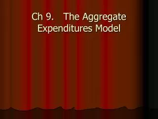
The Income –Expenditure Model • The aggregate expenditures function tells what the economy’s planned spending will be at each level of real GDP. • There will be only one GDP that does match up planned spending and actual spending. • That GDP occurs at the expenditure equilibrium, where the AE function and the 45-degree line intersect.
#2 The 4-degree line shows expenditures by repeating to the vertical axis the real GDP listed on the horizontal axis. #3 At the equilibrium value of GDP, actual spending equals planned spending . #1 The aggregate expenditure function shows how much the economy plans to spend at each possible GDP The Income –Expenditure Model 45o: Spending=production Aggregate Expenditure Function Expenditures $10 trillion $5 trillion $10 trillion Real GDP (income)
Components of Aggregate Expenditures • Spending can be divided into two types: • Autonomous spending: spending that would occur even if people had no income. • Induced spending: spending that depends upon income.
Components of Aggregate Expenditures • Autonomous spending includes both investments and goods. • Draw upon previous wealth and savings. • College students with no earnings drawing down their parents bank accounts to pay for room and board at school. • Graphically, autonomous spending is a positive amount that shows up as a horizontal line.
Components of Aggregate Expenditures • Since induced spending is entirely dependent upon income, graphically it starts at zero starts at zero and GDP rises from there. • When autonomous spending and induced spending are added together, the result is an aggregate expenditure function that has both a positive vertical intercept, and a positive slope.
Aggregates expenditures includes both autonomous and induced spending. Aggregate Expenditure Function Induced spending Autonomous spending Aggregate Expenditures Expenditures $10 trillion $5 trillion 0 $10 trillion Real GDP (income)
Components of Aggregate Expenditures • The components of aggregate expenditures are merely the components of GDP. GDP = C + I + G + (X-M) • The consumption function because of autonomous spending has a positive vertical intercept. • From there, it slopes upward because of the marginal propensity to consume (mpc).
MPC and MPS • The marginal propensity to consume (MPC) is the fraction of additional income that people spend. • The marginal propensity to save (MPS) is the fraction of additional income that people save. MPC + MPS = 1
The Aggregate Expenditures Function • Investment and government purchases are of roughly comparable size. • If planned government purchases and investment spending are assumed to be completely autonomous, they will be constant as GDP changes. • For this reason, the slope of the AE function and the consumption function are the same.
Modeling the Expenditure Equilibrium • When the economy is not at equilibrium, actual GDP and planned spending differ. • Unintended inventory changes show up as the difference between planned and actual investment.
Modeling the Expenditure Equilibrium Expenditure equilibrium: aggregate expenditures = actual GDP where Aggregate expenditures: consumption + planned investment government + net exports and GDP = consumption + actual investment + government +net exports which implies Expenditure equilibrium: planned investment = actual investment
Output decreases but at a decreasing rate. Modeling the Expenditure Equilibrium 45o: Spending=production #1 if the economy starts here #2 A progression of inventory buildups less production leads to the expenditures equilibrium here. Expenditures Aggregate Expenditure Function Real GDP (income)
10.3CHANGING THE EXPENDITURE EQUILIBRIUM • When there are changes in autonomous spending, the changes are magnified by the multiplier effect. • Adding autonomous spending causes a higher GDP, which causes more induced spending. • That’s because money that one person spends autonomously adds to income of others, which in turn induces them to buy more output. • At each stage in this cycle, however, some income is saved, thus eventually bringing the cycle to a halt.
The expenditure equilibrium moves higher Increase in autonomous expenditures Increase in GDP The Multiplier Effect Aggregate expenditure function Expenditures The multiplier effect causes a small increase in autonomous expenditures to have a much larger effect on GDP. Real GDP (income)
The Multiplier Effect • The strength of the multiplier effect depends upon the proportion of income that is devoted to consumption. • To the extent that people save their incomes, savings represents a leakage out of the multiplier process. • A negative value for savings means that there is dissaving – spending out of existing savings.
Spending Depends upon the Marginal Propensity to Consume (mpc):
The Expenditure Multiplier Expenditure multiplier = 1/mps or 1/(1-MPC) Autonomous spending x 1/mps = Expenditure equilibrium
The Multiplier Effect • The multiplier is multiplied by a change in autonomous spending to reveal the change in equilibrium GDP. • There must be some idle resources for the multiplier effect to occur. • Keynesian multiplier analysis assumes a constant price level.
Recession and Inflation within the Income-Expenditure Model • If the expenditure equilibrium lies below full-employment GDP, it is called an unemployment equilibrium. • Along with the unemployment equilibrium comes an output gap, in which actual GDP falls below full-employment GDP. • At an unemployment equilibrium, there is to little spending for the economy to achieve full employment GDP.
Recession and Inflation within the Income-Expenditure Model The shortfall in spending is called a recessionary gap. • If the expenditure equilibrium lies below full-employment GDP, it is called an unemployment equilibrium. • Along with the unemployment equilibrium comes an output gap, in which actual GDP falls below full-employment GDP. • At an unemployment equilibrium, there is to little spending for the economy to achieve full employment GDP.
Recession and Inflation within the Income-Expenditure Model • If the expenditure equilibrium occurs past the full-employment GDP, multiplier analysis does not apply, because inflation will not allow it to stay there. • This possibility is referred to as an inflationary gap, which is the excess of the aggregate expenditure function above that consistent with a full employment equilibrium.
Making Policy with Multipliers • Keynesian analysis suggest that govern can use taxes to stimulate the economy. • However people might save some of their higher after tax income rather than spend it. The tax multiplier, which is the expansionary, or contractionary effect of a tax cut, or increase would be less than the multiplier by the amount of the initial round of spending.
Making Policy with Multipliers Tax Multiplier = -mpc/(1-mpc)
Balanced Budget Multiplier • Keynesians view extra government spending as the most effective policy to cure a recession. • The balanced-budget multiplier combines the expenditure multiplier for an increase in government spending and the tax multiplier because taxes would increase to finance that spending.
Making Policy with Multipliers Balanced Budget Multiplier = 1/(1-mpc) – mpc/(1-mpc)= (1-mpc)/(1-mpc)=1
Aggregate Expenditures with lower price level P1 Aggregate Expenditures with higher price level P2 P2 P1 Aggregate Demand GDP2 GDP1 10.4 AGGREGATE DEMAND 45o: Spending=production Expenditures Actual Real GDP (income) Price Level Real GDP
10.5 EXPLORE & APPLYThe Great Depression • The 1920’s era of prosperity peaked in early 1929. • A few months later the stock market crashed. • The Great Depression began and did not end for over a decade. • Keynesian aggregate expenditure analysis can be used to describe the depression and the policy action to correct it.
income-expenditures model aggregate expenditures aggregate expenditures function expenditure equilibrium autonomous spending induced spending consumption function marginal propensity to consume marginal propensity to save Terms Along the Way
multiplier effect expenditure multiplier unemployment equilibrium output gap recessionary gap inflationary gap tax multiplier balanced budget multiplier Terms Along the Way
Test Yourself • John Maynard Keynes offered a long-run perspective on the macro-economy in the general theory. • If you had no income you could still engage in induced spending. • The marginal propensity to consume must be 1 or less. • An expenditure equilibrium occurs where the aggregate expenditure function intersects the vertical axis. • An injection of new autonomous spending will leave equilibrium real GDP unchanged when the marginal propensity to save equals 0.5.
Test Yourself 2. Suppose actual spending equals planned spending. Then we can say • the economy is at an expenditure equilibrium. • real GDP is the most it can possibly be. • autonomous spending equals zero. • aggregate demand has shifted to the left.
Test Yourself 3. In the income expenditures model the 45-degree line shows • the amount of autonomous spending. • the amount of induced spending. • the expenditure multiplier. • that the economy’s expenditures are actually the same as its output. .
Test Yourself 4. Aggregate expenditures include all of the following except • consumption. • planned investment. • net exports. • unintended changes in business inventories.
Test Yourself 5. The marginal propensity to consume equals • the fraction of their total income that people consume. • the fraction of additional income that people consume. • the fraction of their savings that people plan to spend within the next year. • one in most cases..
Test Yourself 6. The paradox of thrift, if true suggest that people should • save more. • spend more. • vote more often. • spend the same amount of money, but spend it more wisely.
The End! Next Chapter 11 “Fiscal Policy in Action"