Download
1 / 16
160 likes | 337 Vues
Ch 9. The Aggregate Expenditures Model. (a) The investment demand curve and (b) the investment schedule. The level of investment spending ($20 bill) is determined by the interest rate (8%) together with the investment demand curve (ID).

E N D
(a) The investment demand curve and (b) the investment schedule • The level of investment spending ($20 bill) is determined by the interest rate (8%) • together with the investment demand curve (ID). • The investment schedule (Ig) relates the amount of investment ($20 bill) determined • in (a) to the various levels of GDP (set amount/constant).
A. Equilibrium GDP: (GDP = C + Ig). Savings equals planned investment (S=Ig). B. Planned investment – amount firms plan to invest. C. Investment schedule – shows amount firms plan to invest at possible values of real GDP. D. Aggregate expenditures schedule – shows total amount spent on final goods/ services at diff. levels of real GDP.
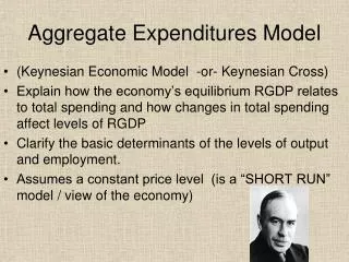
Aggregate Expenditure is a measure of national income. It is a way to measure the totalGDP or Gross Domestic Product (A measure of the level of economic activity). It is defined as the value of planned goods and services produced in an economy. GDP is calculated by the formula C + I + G + NX • C = Consumption Expenditure (Also written as CE) • I = Investment (Ip + Iu planned + unplanned) • G = Government spending • NX = Net exports (Exports-Imports) Aggregate Expenditures is defined as C + Ig. -- John Maynard Keynes (pronounced Caines) developed the Aggregate Expenditures Model, aka the ‘Keynesian Model’ or ‘Keynes Cross.’ -- The amount of goods & services produced and therefore the level of employ- ment depend directly on the level of aggregate expenditures (total spending).
Keynes ideas, called Keynesian economics, had a major impact on the Great Depresison and modern economic / political theory as well as on many gov’ts' fiscal policies. He advocated Interventionist gov’t policy, by which the gov’t would use fiscal and monetary measures to mitigate the adverse effects of economic recessions, depressions and booms. He is one of the fathers of modern theoretical macroeconomics. John Maynard Keynes – British economist favored the heavy gov’t spending during a recession, even running a deficit, to jumpstart the economy (Keynesian economics). Keynes appeared on Dec 31, 1965 edition of TIME magazine. Keynes argued that the solution to depression was to stimulate the economy ("inducement to invest") through some combination of two approaches : A reduction in interest rates. Government investment in infrastructure.
(2) Real Domestic Output (and Income) (GDP=DI) (3) Con- sump- tion (C) (7) Unplanned Changes in Inventories (+ or -) (8) Tendency of Employment Output and Income (5) Investment (Ig) (6) Aggregate Expenditures (C+Ig) (1) Employ- ment (4) Saving (S) (1-2) Consumption and Investment …in Billions of Dollars • 40 • 45 • 50 • 55 • 60 • 65 • 70 • 75 • 80 • 85 $370 390 410 430 450 470 490 510 530 550 $375 390 405 420 435 450 465 480 495 510 $-5 0 5 10 15 20 25 30 35 40 20 20 20 20 20 20 20 20 20 20 $395 410 425 440 455 470 485 500 515 530 $-25 -20 -15 -10 -5 0 +5 +10 +15 +20 Increase Increase Increase Increase Increase Equilibrium Decrease Decrease Decrease Decrease The table shows 10 possible levels of production. Graphically…
530 510 490 470 450 430 410 390 370 Consumption (billions of dollars) 45° • 390 410 430 450 470 490 510 530 550 Disposable Income (billions of dollars) Consumption and Investment Equilibrium GDP C + Ig (C + Ig = GDP) C Equilibrium Point Aggregate Expenditures The Keynesian Model (Keynes Cross) showing the Aggregate Expenditure Model Ig = $20 Billion C = $450 Billion
Equilibrium GDP: C + Ig = GDP • Aggregate expenditures – in a closed economy, AE consists of C (col 3) + I (col 5) = sum in col 6. Col 2 makes the AE schedule (GDP=DI). • The schedule shows the amount (C+Ig) that will be spent at each possible output or income level. • Equilibrium GDP where GDP (DI) & AE columns are equal (col. 2 and 6, are each $470 bill).
Equilibrium Graph Changes in the equilibrium GDP caused by shifts in the aggregate expenditures schedule and the investment schedule Equilibrium point C+Ig C Increase in investment The Keynes Cross showing the Aggregate Expenditure Model ● 470 Aggregate expenditures Decrease in investment 450 470 450 Real domestic product, GDP
E. Multiplier: Δ in output & income Δ in investment spending • If the amount invested increased by $5 billion, that increase will shift the graph upward. • $5 billion Δ in investment spending leads to $20 billion Δ in output & income (income is Y). • Multiplier is 4 (= $20/$5). • MPS is .25
In an open-mixed economy, equilibrium GDP occurs where: Ca+Ig+Xn+G=GDP
Net exports and equilibrium GDP Net exports are exports minus imports.
c Gov’t spending and equilibrium GDP Gov’t spending increase b ● d ● e a Aggregate expenditures Real GDP Point ‘a’ -- In a private closed economy, the APC is equal to 1 at what income level? -- If AE are Ca+Ig+Xn+G, the amount of savings at $225 are what points? Points ‘c and d”
550 530 510 490 470 Aggregate Expenditures (billions of dollars) 45° 490 510 530 Real GDP (billions of dollars) Equilibrium Versus Full-Employment GDP Recessionary Expenditure Gap AE0 $5 Billion Gap Yields $20 Billion GDP Change AE1 Recessionary Expenditure Gap = $5 Billion Full Employment
550 530 510 490 470 Aggregate Expenditures (billions of dollars) 45° 490 510 530 Real GDP (billions of dollars) Equilibrium Versus Full-Employment GDP Inflationary Expenditure Gap AE2 AE0 Inflationary Expenditure Gap = $5 Billion $5 Billion Gap Yields $20 Billion GDP Change Full Employment
F. Lump-sum tax – tax that’s a constant amount at all levels of GDP. G. Recessionary gap – amount the agg expenditures schedule must shift upward to increase real GDP to full-employment. H. Inflationary gap – amount the agg expenditures schedule must shift downward to decrease real GDP to full- employment. Opposites