Download
1 / 24
240 likes | 267 Vues
T MVA A Multivariate Analysis Toolkit. Andreas H öcker, Jörg Stelzer , Fredrik Tegenfeldt, Helge Voss Core Developers Matthew Jachowski, Attila Krasznahorkay, Yahir Mahalalel, Xavier Prudent, Peter Speckmayer Contributors. – Introduction –.

E N D
TMVAA Multivariate Analysis Toolkit Andreas Höcker, Jörg Stelzer, Fredrik Tegenfeldt, Helge Voss Core Developers Matthew Jachowski, Attila Krasznahorkay, Yahir Mahalalel, Xavier Prudent, Peter Speckmayer Contributors
– Introduction – • Event classification is main objective of data mining in HEP • Signal vs background event separation, particle ID, flavor-tagging, … • Can have many input variables (between ~10 to ~50), often correlated • Many classification methods exist and are already used in HEP (BABAR almost all analysis use MVA methods) • HEP tradition: rectangular cuts (with previous de-correlation) optimization often by hand • Also widely accepted: Likelihood (usually in one or two dimensions only) • Somewhat new: multidimensional Probability Density Estimators – range search • Gaining Trust: Artificial Neural Networks • Simple, but can be powerful: Fisher Discriminant (BABAR, BELLE: B selection) • Newcomers: Boosted Decision Trees (MiniBoone, D0) • Powerful new method from Friedman: Rulefit (Study at ATLAS) • Uprising: Support Vector Machines (studies for LEP andTevatron top analysis) • Two Problems • Skepticism: black box myth, how to evaluate systematics • Choice of method: by simplicity, availability, hearsay, limited comparison Jörg Stelzer
– What is TMVA – TMVA • Ideally, for a given problem all MVA methods should be tested • Systematically chose the best performing classifier • Becoming familiar and gaining experience with other MVA methods takes away the mysticism • TMVA – Toolkit for Multivariate Analysis: • Framework for parallel training and evaluation of MVA techniques to guide the user to choose of the best signal-background discriminator for his purpose • TMVA does not seek to promote any particular classifier, the judgment isup to the user • Currently Supported Methods • Cuts (optimizers: MC sampling, Genetic alg, simulated annealing) • 1-dimensional Likelihood Estimator • Multi-dimensional Probability Density Estimator (range search) • Fisher Discriminant (also H-matrix (χ2-estimator)) • Artificial Neural Network (3 different implementations) • Boosted/bagged Decision Trees • Rulefit • Transformation of input variables: decorrelation, PCA Jörg Stelzer
– What does TMVA do Exactly – • The analyst provides: • Training and testing data for signal and background • ROOT tree of text file with events • List of variables to be included in the analysis • List of MVA methods to be used • TMVA analysis provides: • Training, testing and evaluating all user-selected MVA-methods • Graphical and numerical evaluation available guide user’s choice • Ranking of input variables • Preliminary general ranking • Method specific ranking • Training results are written to self-contained ‘weight’-files • Weight files also contain the complete training setup of a method • Easy to share an analysis setup with colleagues ! • no need to send code fragments and explanations back and forth • For data analysis (after successful training and selection of MVA) weight file is used by TMVA::Reader class for classification Jörg Stelzer
– TMVA Development and Distribution – • TMVA is a sourceforge (SF) package to accommodate world-wide access • home page …………………..http://tmva.sourceforge.net/ • SF project page ……………..http://sourceforge.net/projects/tmva • view CVS …………………….http://tmva.cvs.sourceforge.net/tmva/TMVA/ • mailing lists …………………..http://sourceforge.net/mail/?group_id=152074 • ROOT::TMVA class index…..http://root.cern.ch/root/htmldoc/TMVA_Index.html • Very active project fast response time on feature requests (or bug reports) • Currently 4 main developers at CERN, ~23 registered contributors at SF • Written in C++ using core ROOT functionality • Integrated and distributed with ROOT since ROOT v5.11-03 • Available out of the box (ROOT is everywhere) • Only thoroughly tested TMVA versions in ROOT • Always with up-to-date example in $ROOTSYS/tmva/test/ • Documentation currently being written, release date next week Jörg Stelzer
– TMVA Technical Details – • TMVA can be used • C++ executable: (athena), examples SourceForge • CINT macros: examples at $ROOTSYS/tmva/test/ • Python (PyROOT), example only at SourceForge • Modular • Can switch on/off each method • Simultaneously train multiple instances of one method with different options • Flexible • Configuration of methods through custom option strings • Input variables (can be formulas as in TTree::Draw command) • Arrays are handled (“p”), but not array indices at present (“p[0]”) • User friendly • Option names easy to interpret • Default options are already good choice to start with • Graphical training and evaluation output (macros provided) • Once trained, classification to real data straight forward • C++/CINT example at $ROOTSYS/tmva/test/TMVApplication.C Jörg Stelzer
The Methods inTMVA Jörg Stelzer
Decorrelation of Input Variables • Cuts and projective likelihood perform best/optimal if there is no correlation between input variables • Remove linear correlations between input variables by rotation of parameter space • Separate transformation for signal and background • De-correlation only complete if • input variables are Gaussian • Correlations are linear • In practice the gain is often only modest Diagonalize (S) the covariance matrix CD Transform (ST) the square root of D C’ Decorrelate input space x with C’-1 x’ Jörg Stelzer
Cuts • Intuitive and most simple method: cut a rectangular volume out of parameter space that defines the signal • Training samples do often not contain realistic signal and background abundance no direct optimization for significance • Instead scan signal efficiency [0,1] and maximize background rejection • Straight forward computation of optimal working point (highest significance) given S and B expectation • Cut optimization: • MINUIT fit (simplex) was found not to be reliable • Three different (robust) methods • Monte Carlo sampling: • random scanning of parameter space • inefficient for large number of input variables • Genetic algorithm: Preferred method • Samples of cut-sets (a population) are evaluated and the fittest individuals are cross-bred (including mutation) to create the new generation • Simulated annealing: still need to optimize its performance • slow cooling of a metal makes atoms move into lowest energy state, simulated by a energy dependent perturbation probability to recover from local minima Jörg Stelzer
Projected Likelihood Estimator • Probability density functions for all variables combined (for signal and for background) to form likelihood-ratio estimator • Optimal MVA approach, if variables are uncorrelated • In practice rarely the case, solution: de-correlate input or use different method • Reference PDFs are automatically generated from training data and represented as histograms (counting) or splines (order 2,3,5) – unbinned kernel estimator in work • Output of likelihood estimator often strongly peaked at 0 and 1. To ease output parameterization TMVA applies inverse Fermi transformation. Reference PDF Jörg Stelzer
Multidimensional PDE • Extend the one-dimensional approach to n dimensions (n – number of input variables) • Carli-Koblitz Range-Search:Searches a volume around event and counts(&weights) signal and background reference events (training sample) this volume (nS/B) • Volume: • Size: can be fixed (defined by the data: % of Max-Min or RMS) or adaptive (define by number of events in search volume) • Shape: box or ellipsoid • Weights as function of the (normalized) distance between test- and reference events in volume can be applied (linear or Gaussian) • Practical challenges: • Need very large training sample (curse of dimensionality of kernel based methods) • Fast training, slow evaluation. • Speed up range search by sorting reference sample into binary search trees Jörg Stelzer
Linear Fisher Discriminant • Well-known, simple and elegant MVA method • Linear discriminant analysis determines a axis in the input variable hyperspace (F1,…,Fn, such that a projection of events on this axis pushes signal and background as far away from each other as possible • Optimal for linearly correlated Gaussian variables where S and B have different means • No separation power from variables v with different shapes but the same mean Fv=0 • H-matrix estimator: poor man’s variation of Fisher discriminant W: sum of S and B covariance matrices Fisher Coefficient Jörg Stelzer
Artificial Neural Network (ANN) Typical activation function y’j w0 v’j v0 v1 vn y’j y0 yn y1 w1 . . . wn v’j • ANNs are non-linear discriminants • Non linearity from activation function. (Fisher is an ANN with linear activation function) • Multilayer perceptron: fully connected, feed forward, 1..NH hidden layers • Can approximate every continuous function to arbitrary precision withjust one layer and infinite nodes (Weierstrass) • Training of an MLP: back-propagation method • Randomly feed signal and background events to MLP and compare the desired output {0,1} with the received output (0,1): ε = d - r • Correct weights, depending on ε and learning rate η Jörg Stelzer
(Boosted) Decision Trees S,B S2,B2 S1,B1 • Tree structure classifier (S and B leafs) • Classifies events by following a sequence of decisions depending on the events variable content until a S or B leaf • Training the tree: e.g. split minimizes Gini-index • other splitting criteria: significance, cross-entropy, misclassification error • Decision trees are robust in many dimensions but by itself not powerful (similar to cuts) Need to boost • Method to combine classifiers: boosting(also implemented: bagging) • Developed by statisticians in last decade • Boosting: (Adaboost) • Re-weight events, higher weight for misclassified events, lower for correctly classified events • Retrain and repeat set of classifiers • Classify data by a weighted vote of the classifiers ROOT-Node S,B Node S2,B2 Leaf-Node S1 < B1 Bkg Leaf-Node S4 > B4 Signal Node S3,B3 Leaf-Node S5 < B5 Bkg Leaf-Node S6 > B6 Signal Jörg Stelzer
Rulefitter • New and powerful method of J.Friedman • Belongs to the class of combined classifiers • This one combines decision trees from a ‘random forest’ • Also adds a linear discriminant (Fisher) term • Random subsets of training data used to create random forest of decision trees (ym) • Coefficients am are then fitted • Friedman, Popescu, “Gradient Directed Regularization for Linear Regression and Classification”, Technical report, statistics department, Stanford University 2003 Jörg Stelzer
HOWTO useTMVA Jörg Stelzer
– Training (from TMVAnalysis.C) – Create the Factory Tell the Factory about your data Book desired methods/options Perform training and evaluation Open the GUI for performance plots // create the root output file TFile* target = TFile::Open( "TMVA.root", "RECREATE" ); // create the factory object TMVA_Factory *factory = new TMVA_Factory( “Project", target, "" ); --- Factory : Evaluation results ranked by best 'signal eff @B=0.10' --- Factory : ----------------------------------------------------------------------------- --- Factory : MVA Signal efficiency (error): Signifi- Sepa- mu-Trans- --- Factory : Methods: @B=0.01 @B=0.10 @B=0.30 cance: ration: form: --- Factory : ----------------------------------------------------------------------------- --- Factory : Fisher : 0.292(07) 0.690(07) 0.900(04) 1.261 0.484 0.991 --- Factory : LikelihoodPCA : 0.245(06) 0.684(07) 0.896(04) 1.330 0.477 0.867 --- Factory : MLP : 0.287(07) 0.682(07) 0.903(04) 1.328 0.483 0.991 --- Factory : LikelihoodD : 0.287(07) 0.673(07) 0.898(04) 1.331 0.480 0.861 --- Factory : HMatrix : 0.075(04) 0.663(07) 0.884(05) 1.179 0.451 0.991 --- Factory : PDERS : 0.225(06) 0.646(07) 0.878(05) 1.258 0.449 0.911 --- Factory : BDT : 0.200(06) 0.641(07) 0.872(05) 1.219 0.432 0.991 --- Factory : RuleFit : 0.245(06) 0.632(07) 0.882(05) 1.246 0.451 0.901 --- Factory : CutsGA : 0.262(06) 0.622(07) 0.868(05) 0.000 0.000 0.000 --- Factory : Likelihood : 0.155(05) 0.538(07) 0.810(06) 0.983 0.353 0.767 --- Factory : ----------------------------------------------------------------------------- --- Factory : --- Factory : Testing efficiency compared to training efficiency (overtraining check) --- Factory : ----------------------------------------------------------------------------- --- Factory : MVA Signal efficiency: from test sample (from traing sample) --- Factory : Methods: @B=0.01 @B=0.10 @B=0.30 --- Factory : ----------------------------------------------------------------------------- --- Factory : Fisher : 0.292 (0.235) 0.690 (0.655) 0.900 (0.892) --- Factory : LikelihoodPCA : 0.245 (0.222) 0.684 (0.677) 0.896 (0.891) --- Factory : MLP : 0.287 (0.232) 0.682 (0.661) 0.903 (0.895) --- Factory : LikelihoodD : 0.287 (0.245) 0.673 (0.664) 0.898 (0.889) --- Factory : HMatrix : 0.075 (0.058) 0.663 (0.645) 0.884 (0.877) --- Factory : PDERS : 0.225 (0.335) 0.646 (0.674) 0.878 (0.884) --- Factory : BDT : 0.200 (0.240) 0.641 (0.750) 0.872 (0.892) --- Factory : RuleFit : 0.245 (0.242) 0.632 (0.621) 0.882 (0.872) --- Factory : CutsGA : 0.262 (0.183) 0.622 (0.607) 0.868 (0.861) --- Factory : Likelihood : 0.155 (0.137) 0.538 (0.526) 0.810 (0.797) --- Factory : ----------------------------------------------------------------------------- TFile * input = TFile::Open("tmva_example.root"); TTree *signal = (TTree*)input->Get("TreeS"); TTree *background = (TTree*)input->Get("TreeB"); factory->SetInputTrees( signal, background, sWeight, bWeight); factory->AddVariable("var1+var2",'F');factory->AddVariable(“var1-var2",'F'); factory->AddVariable("var3", 'F'); factory->AddVariable("var4", 'F'); factory->BookMethod( TMVA::Types::kCuts, "CutsD", "!V:MC:EffSel:MC_NRandCuts=200000:VarTranform=Decorrelate" ); factory->BookMethod( TMVA::Types::kLikelihood, "LikelihoodPCA", "!V:!TransformOutput:Spline=2:NSmooth=5:VarTransform=PCA"); User chooses the best method // Train all configured MVAs using the set of training events factory->TrainAllMethods(); // Evaluate all configured MVAs using the set of test events factory->TestAllMethods(); // Evaluate and compare performance of all configured MVAs factory->EvaluateAllMethods(); // open the GUI for the root macros TMVAGui(); Jörg Stelzer
– Application (from TMVApplication.C) – Create the Reader Declare the variables that will hold your data Chose the MVA method you like best Prepare the user data Analyze the user data, fill histogram, etc. // create the Reader object TMVA::Reader *reader = new TMVA::Reader(); // create a set of variables and declare them to the reader Float_t var1, var2, var3, var4; reader->AddVariable( "var1+var2", &var1 ); reader->AddVariable( "var1-var2", &var2 ); reader->AddVariable( "var3", &var3 ); reader->AddVariable( "var4", &var4 ); reader->BookMVA( "BDT method", “weigths/Project_BDT.weights.txt" ); TTree* theTree = (TTree*)input->Get("TreeS"); Float_t userVar1, userVar2; theTree->SetBranchAddress( "var1", &userVar1 ); theTree->SetBranchAddress( "var2", &userVar2 ); theTree->SetBranchAddress( "var3", &var3 ); theTree->SetBranchAddress( "var4", &var4 ); Use for further analysis (Fit for signal yield, systematic studies, etc.) // loop over user data for (Long64_t ievt=0; ievt<theTree->GetEntries();ievt++) { theTree->GetEntry(ievt); var1 = userVar1 + userVar2; var2 = userVar1 - userVar2; histBdt ->Fill( reader->EvaluateMVA( "BDT method") ); } Jörg Stelzer
TMVA– an example Jörg Stelzer
– Toy Example – Also with SF and ROOT – • Simple toy to illustrate the strength of the de-correlation technique • 4 linearly correlated Gaussians, with equal RMS and shifted means between signal and background All plots from GUI Jörg Stelzer
Decorrelation of Training Input • Scatter plot pf all pairs of input variables (and profile) • Decorrelation procedure can be applied before training Jörg Stelzer
Likelihood and Cuts Improvement • On linearly correlated variables Fisher is already the optimum • Decorrelation of input: LH and Cuts comparable with Fisher Jörg Stelzer
More Information All MVA outputs LH reference distributions BDT visual ANN information Jörg Stelzer
Summary • TMVA is now a mature package • User feedback from many HEP collaborations (including neutrino physics) • Integration into ROOT essential • Emphasis on consolidating and improving current methods as well as the TMVA framework • Providing user interface to Athena (AOD, EventView analyses) • Standalone application of methods • New methods are being developed • Support vector machine • Bayesian Classifier • Committee method • Optimizes arbitrary combinations of MVA methods Jörg Stelzer