Multivariate Data Analysis with T MVA

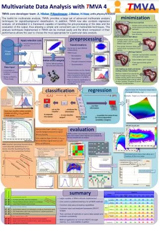
Multivariate Data Analysis with TMVA Andreas Hoecker(*) (CERN) SOS, Strasbourg, France, July 4, 2008 (*) On behalf of the present core team: A. Hoecker, P. Speckmayer, J. Stelzer, H. Voss And the contributors: A. Christov, Or Cohen, Kamil Kraszewski, Krzysztof Danielowski, S. Henrot-Versillé, M. Jachowski, A. Krasznahorkay Jr., Maciej Kruk, Y. Mahalalel, R. Ospanov, X. Prudent, A. Robert, F. Tegenfeldt, K. Voss, M. Wolter, A. Zemla See acknowledgments on page 43 On the web: http://tmva.sf.net/ (home), https://twiki.cern.ch/twiki/bin/view/TMVA/WebHome (tutorial)

x2 x2 x2 H1 H1 H1 H0 H0 H0 x1 x1 x1 Event Classification • Suppose data sample with two types of events: H0, H1 • We have found discriminating input variables x1, x2, … • What decision boundary should we use to select events of type H1? Rectangular cuts? A linear boundary? A nonlinear one? • How can we decide this in an optimal way ?  Let the machine learn it ! Low variance (stable), high bias methods High variance, small bias methods A. Hoecker: Multivariate Analysis with TMVA

Multivariate Event Classification • All multivariate classifiers have in common to condense (correlated) multi-variable input information in a single scalar output variable • It is a RnR regression problem; classification is in fact a discretised regression y(H0)  0, y(H1)  1 MV regression is also interesting ! In work for TMVA. … A. Hoecker: Multivariate Analysis with TMVA

Event Classification in High-Energy Physics (HEP) • Most HEP analyses require discrimination of signal from background: • Event level (Higgs searches, …) • Cone level (Tau-vs-jet reconstruction, …) • Track level (particle identification, …) • Lifetime and flavour tagging (b-tagging, …) • Parameter estimation (CP violation in B system, …) • etc. • The multivariate input information used for this has various sources • Kinematic variables (masses, momenta, decay angles, …) • Event properties (jet/lepton multiplicity, sum of charges, …) • Event shape (sphericity, Fox-Wolfram moments, …) • Detector response (silicon hits, dE/dx, Cherenkov angle, shower profiles, muon hits, …) • etc. • Traditionally few powerful input variables were combined; new methods allow to use up to 100 and more variables w/o loss of classification power A. Hoecker: Multivariate Analysis with TMVA

T M V A TM V A • Outline of this presentation: • The TMVA project • Overview of available classifiers and processing steps • Evaluation tools • (Toy) examples A. Hoecker: Multivariate Analysis with TMVA

What is TMVA • ROOT: is the analysis framework used by most (HEP)-physicists • Idea: rather than just implementing new MVA techniques and making them available in ROOT (i.e., like TMulitLayerPercetron does): • Have one common platform / interface for all MVA classifiers • Have common data pre-processing capabilities • Train and test all classifiers on same data sample and evaluate consistently • Provide common analysis (ROOT scripts) and application framework • Provide access with and without ROOT, through macros, C++ executables or python A. Hoecker: Multivariate Analysis with TMVA

TMVA Development and Distribution • TMVA is a sourceforge (SF) package for world-wide access • Home page ………………. http://tmva.sf.net/ • SF project page …………. http://sf.net/projects/tmva • View CVS ………………… http://tmva.cvs.sf.net/tmva/TMVA/ • Mailing list .……………….. http://sf.net/mail/?group_id=152074 • Tutorial TWiki ……………. https://twiki.cern.ch/twiki/bin/view/TMVA/WebHome • Active project  fast response time on feature requests • Currently 4 core developers, and 16 active contributors • >2500 downloads since March 2006 (not accounting CVS checkouts and ROOT users) • Written in C++, relying on core ROOT functionality • Integrated and distributed with ROOT since ROOT v5.11/03 A. Hoecker: Multivariate Analysis with TMVA

Limitations of TMVA • Development started beginning of 2006 – a mature but not a final package • Known limitations / missing features • Performs classification only, and only in binary mode: signal versus background • Supervised learning only (no unsupervised “bump hunting”) • Relatively stiff design – not easy to mix methods, not easy to setup categories • Cross-validation not yet generalised for use by all classifiers • Optimisation of classifier architectures still requires tuning “by hand” • Work ongoing in most of these areas  see later in this talk A. Hoecker: Multivariate Analysis with TMVA

T M V A C o n t e n t • Currently implemented classifiers ( see H. Prosper’s lecture) • Rectangular cut optimisation • Projective and multidimensional likelihood estimator • k-Nearest Neighbor algorithm • Fisher and H-Matrix discriminants • Function discriminant • Artificial neural networks (3 multilayer perceptron implementations) ( see J. Schwindling’s lecture) • Boosted/bagged decision trees ( see Y. Coadou’s lecture) • RuleFit • Support Vector Machine • Currently implemented data preprocessing stages: • Decorrelation • Principal Value Decomposition • Transformation to uniform and Gaussian distributions (coming soon) A. Hoecker: Multivariate Analysis with TMVA

D a t a P r e p r o c e s s i n g A. Hoecker: Multivariate Analysis with TMVA

Data Preprocessing: Decorrelation • Commonly realised for all methods in TMVA (centrally in DataSet class) • Removal of linear correlations by rotating input variables • Cholesky decomposition: determine square-rootCof covariance matrixC, i.e.,C = CC • Transform original(x)into decorrelated variable space(x)by:x = C1x • Principal component analysis • Variable hierarchy: linear transformation projecting on axis to achieve largest variance PC of variablek Sample means Eigenvector • Matrix of eigenvectors V obeys relation: thus PCA eliminates correlations A. Hoecker: Multivariate Analysis with TMVA

Data Preprocessing: Decorrelation SQRT derorr. PCA derorr. original • Note that decorrelation is only complete, if • Correlations are linear • Input variables are Gaussian distributed • Not very accurate conjecture in general A. Hoecker: Multivariate Analysis with TMVA

“Gaussian-isation” • Improve decorrelation by pre-Gaussianisation of variables • First: “Rarity” transformation to achieve uniform distribution: Rarity transform of variablek Measured value PDF of variable k • The integral can be solved in an unbinned way by event counting, or by creating non-parametric PDFs (see later for likelihood section) • Second: make Gaussian via inverse error function: A. Hoecker: Multivariate Analysis with TMVA

“Gaussian-isation” Original Signal - Gaussianised Background - Gaussianised We cannot simultaneously Gaussianise both signal and background ?! A. Hoecker: Multivariate Analysis with TMVA

How to apply the Preprocessing Transformation ? • Any type of preprocessing will be different for signal and background • But: for a given test event, we do not know the species ! • Not so good solution: choose one or the other, or a S/B mixture. As a result, none of the transformations will be perfect • Good solution: for some methods it is possible to test both S and B hypotheses with their transformations, and to compare them. Example, projective likelihood ratio: A. Hoecker: Multivariate Analysis with TMVA

T h e C l a s s i f i e r s A. Hoecker: Multivariate Analysis with TMVA

Rectangular Cut Optimisation • Simplest method: cut in rectangular variable volume • Cuts usually benefit from prior decorrelation of cut variables • Technical challenge: how to find optimal cuts ? • MINUIT fails due to non-unique solution space • TMVA uses: Monte Carlo sampling, Genetic Algorithm, Simulated Annealing • Huge speed improvement of volume search by sorting events in binary tree A. Hoecker: Multivariate Analysis with TMVA

( d i g r e s s i o n • minimisation techniques • binary tree sorting A. Hoecker: Multivariate Analysis with TMVA

Minimisation • Robust global minimum finder needed at various places in TMVA • Brute force method: Monte Carlo Sampling • Sample entire solution space, and chose solution providing minimum estimator • Good global minimum finder, but poor accuracy • Default solution in HEP: (T)Minuit/Migrad[ How much longer do we need to suffer …. ? ] • Gradient-driven search, using variable metric, can use quadratic Newton-type solution • Poor global minimum finder, gets quickly stuck in presence of local minima • Specific global optimisers implemented in TMVA: • Genetic Algorithm: biology-inspired optimisation algorithm • Simulated Annealing: slow “cooling” of system to avoid “freezing” in local solution • TMVA allows to chain minimisers • For example, one can use MC sampling to detect the vicinity of a global minimum, and then use Minuit to accurately converge to it. A. Hoecker: Multivariate Analysis with TMVA

Initialisation Population of randomly created individuals Evaluation Compute fitness for each individual Selection Keep fittest individuals according to probability Reproduction Survivors are mutated and crossed over  new population Termination Finish after maximum of generations reached Evolution stages of a genetic algorithm Genetic Algorithm • Algorithm to find approximate solutions to optimisation problems • The problem is modeled by a group (population) of abstract representations (genomes) of possible solutions (individuals). By applying means similar to processes found in biological evolution the individuals of the population should evolve towards an optimal solution of the problem. • Processes which are usually modeled in evolutionary algorithms — of which Genetic Algorithms are a subtype — are inheritance, mutation and “sexual recombination” (also termed crossover). • Apart from the abstract representation of the solution domain, a fitness function must be defined. Its purpose is the evaluation of the goodness of an individual. The fitness function is problem dependent. For example, it could be a negative 2 function. A. Hoecker: Multivariate Analysis with TMVA

Simulated Annealing • Algorithm to find approximate solutions to optimisation problems • When first heating and then slowly cooling down (“annealing”) a metal its atoms move towards a state of lowest energy, while for sudden cooling the atoms tend to freeze in intermediate higher energy states. • For infinitesimal annealing activity the system will always converge in its global energy minimum. • This physical principle can be simulated to achieve slow, but correct convergence of an optimisation problem with multiple solutions. • Recovery out of local minima is achieved by assigning the probability • to a perturbation of a parameter. Lowering the temperature diminishes the probability of bad perturbations to occur. Change in 2 by new solution Annealing temperature of system A. Hoecker: Multivariate Analysis with TMVA

Simulated Annealing – Example Example illustrating the effect of cooling schedule on the performance of simulated annealing. The problem is to rearrange the pixels of an image so as to minimise a certain potential energy function, which causes similar colours to attract at short range and repel at slightly larger distance. The elementary moves swap two adjacent pixels. The images were obtained with fast cooling schedule (1st) and slow cooling schedule (2nd), producing results similar to amorphous and crystalline solids, respectively. Source: http://en.wikipedia.org/wiki/Simulated_annealing A. Hoecker: Multivariate Analysis with TMVA

Minimisation Techniques Grid search Quadratic Newton Simulated Annealing Source: http://www-esd.lbl.gov/iTOUGH2/Minimization/minalg.html A. Hoecker: Multivariate Analysis with TMVA

Binary Trees • Tree data structure in which each node has at most two children • Typically the child nodes are called left and right • Binary trees are used in TMVA to implement binary search trees and decision trees Root node < > • Amount of computing time to search for events: • Box search:  (Nevents)Nvar • BT search:  Nevents·Nvarln2(Nevents) Depth of a tree Leaf node A. Hoecker: Multivariate Analysis with TMVA

) A. Hoecker: Multivariate Analysis with TMVA

Projective Likelihood Estimator (PDE Approach) • Much liked in HEP: probability density estimators for each input variable combined in likelihood estimator Likelihood ratio for event ievent PDFs discriminating variables PDE introduces fuzzy logic Species: signal, background types • Ignores correlations between input variables • Optimal approach if correlations are zero (or linear  decorrelation) • Otherwise: significant performance loss A. Hoecker: Multivariate Analysis with TMVA

PDE Approach: Estimating PDF Kernels • Technical challenge: how to estimate the PDF shapes • 3 ways: parametric fitting (function)nonparametric fitting event counting Difficult to automate for arbitrary PDFs Easy to automate, can create artefacts/suppress information Automatic, unbiased, but suboptimal • We have chosen to implement nonparametric fitting in TMVA original distribution is Gaussian • Binned shape interpolation using spline functions and adaptive smoothing • Unbinned adaptive kernel density estimation (KDE) with Gaussian smearing • TMVA performs automatic validation of goodness-of-fit A. Hoecker: Multivariate Analysis with TMVA

Multidimensional PDE Approach • Use a single PDF per event class (sig, bkg), which spans Nvar dimensions • PDE Range-Search: count number of signal and background events in “vicinity” of test event  preset or adaptive volume defines “vicinity” Carli-Koblitz, NIM A501, 576 (2003) • The signal estimator is then given by (simplified, full formula accounts for event weights and training population) • Variant: k-Nearest Neighbor– implemented by R. Ospanov(Texas U.): • Better than searching within a volume (fixed or floating), count adjacent reference events till statistically significant number reached • Method intrinsically adaptive • Very fast search with kd-tree event sorting x2 H1 Metric ? PDE-RS ratio for event ievent chosen volume #signal events in V test event H0 #background events in V x1 If volume too small: overtraining, if too big: loss of sensitivity • Improve yPDERS estimate within V by using various Nvar-D kernel estimators Best method when very large training sample available (but slow!) • Enhance speed of event counting in volume by binary tree search A. Hoecker: Multivariate Analysis with TMVA

Fisher’s Linear Discriminant Analysis (LDA) • Well known, simple and elegant classifier • LDA determines axis in the input variable hyperspace such that a projection of events onto this axis pushes signal and background as far away from each other as possible, while confining events of same class in close vicinity to each other • Function discriminant analysis (FDA) • Fit any user-defined function of input variables requiring that signal events return 1 and background 0 • Parameter fitting: Genetics Alg., MINUIT, MC and combinations • Easy reproduction of Fisher result, but can add nonlinearities • Very transparent discriminator • Classifier response couldn’t be simpler: “Fisher coefficients” “Bias” • Compute Fisher coefficients from signal and background covariance matrices • Fisher requires distinct sample means between signal and background • Optimal classifier (Bayes limit) for linearly correlated Gaussian-distributed variables A. Hoecker: Multivariate Analysis with TMVA

1 input layer k hidden layers 1 ouput layer ... 1 1 1 2 output classes (signal and background) . . . . . . . . . Nvar discriminating input variables i j Mk . . . . . . N M1 (“Activation” function) with: Nonlinear Analysis: Artificial Neural Networks • Achieve nonlinear classifier response by “activating” output nodes using nonlinear weights Weierstrass theorem: can approximate any continuous functions to arbitrary precision with a single hidden layer and an infinite number of neurons Feed-forward Multilayer Perceptron Weight adjustment using analytical back-propagation (stochastic minimisation) • Three different implementations in TMVA (all are Multilayer Perceptrons) • TMlpANN: Interface to ROOT’s MLP implementation ( see J. Schwindling’s talk) • MLP: TMVA’s own MLP implementation for increased speed and flexibility • CFMlpANN: ALEPH’s Higgs search ANN, translated from FORTRAN A. Hoecker: Multivariate Analysis with TMVA

Decision Trees • Sequential application of cuts splits the data into nodes, where the final nodes (leafs) classify an event assignalorbackground • Growing a decision tree: • Start with Root node • Split training sample according to cut on best variable at this node • Splitting criterion: e.g., maximum “Gini-index”: purity  (1– purity) • Continue splitting until min. number of events or max. purity reached • Classify leaf node according to majority of events, or give weight; unknown test events are classified accordingly Decision tree after pruning Decision tree before pruning • Bottom-up “pruning” of a decision tree • Why not multiple branches (splits) per node ? • Remove statistically insignificant nodes to reduce tree overtraining • Fragments data too quickly; also: multiple splits per node = series of binary node splits A. Hoecker: Multivariate Analysis with TMVA

Boosted Decision Trees (BDT) • Data mining with decision trees is popular in science (so far mostly outside of HEP) • Advantages: • Independent of monotonous variable transformations, immune against outliers • Weak variables are ignored (and don’t (much) deteriorate performance) • Shortcomings: • Instability: small changes in training sample can dramatically alter the tree structure • Sensitivity to overtraining ( requires pruning) • Boosted decision trees: combine forest of decision trees, with differently weighted events in each tree (trees can also be weighted), by majority vote • e.g., “AdaBoost”: incorrectly classified events receive larger weight in next decision tree • “Bagging” (instead of boosting): random event weights, resampling with replacement • Boosting or bagging are means to create set of “basis functions”: the final classifier is linear combination (expansion) of these functions improves stability ! A. Hoecker: Multivariate Analysis with TMVA

Predictive Learning via Rule Ensembles (RuleFit) Friedman-Popescu, Tech Rep, Stat. Dpt, Stanford U., 2003 • Following RuleFit approach by Friedman-Popescu • Model is linear combination of rules, where a rule is a sequence of cuts RuleFit classifier rules (cut sequence  rm=1 if all cuts satisfied, =0 otherwise) normalised discriminating event variables Sum of rules Linear Fisher term • The problem to solve is • Create rule ensemble: use forest of decision trees • Fit coefficients am, bk: gradient direct regularization minimising Risk (Friedman et al.) • Pruning removes topologically equal rules” (same variables in cut sequence) One of the elementary cellular automaton rules (Wolfram 1983, 2002). It specifies the next color in a cell, depending on its color and its immediate neighbors. Its rule outcomes are encoded in the binary representation 30=000111102. A. Hoecker: Multivariate Analysis with TMVA

Support Vector Machine (SVM) • Find hyperplane that best separates signal from background x2 support vectors • Best separation: maximum distance (margin) between closest events (support) to hyperplane • Linear decision boundary • Solution of Lagrangian only depends on inner product of support vectors 1 Non-separable data 2 Separable data optimal hyperplane 3 4 margin • If data non-separable add misclassification costparameter C·ii to minimisation function x1 A. Hoecker: Multivariate Analysis with TMVA

x3 x2 x2 x1 x1 x1 Support Vector Machine (SVM) • Find hyperplane that best separates signal from background • Best separation: maximum distance (margin) between closest events (support) to hyperplane • Linear decision boundary • Solution of Lagrangian only depends on inner product of support vectors (x1,x2) • If data non-separable add misclassification costparameter C·ii to minimisation function • Non-linear cases: • Transform variables into higher dimensional feature space where again a linear boundary (hyperplane) can separate the data • Explicit basis functions not required: use Kernel Functions to approximate scalar products between transformed vectors in the higher dimensional feature space • Choose Kernel and fit the hyperplane using the linear techniques developed above • Available Kernels:Gaussian, Polynomial, Sigmoid A. Hoecker: Multivariate Analysis with TMVA

U s i n g T M V A • A typical TMVA analysis consists of two main steps: • Trainingphase: training, testing and evaluation of classifiers using data samples with known signal and background composition • Application phase: using selected trained classifiers to classify unknown data samples • Illustration of these steps with toy data samples TMVA tutorial A. Hoecker: Multivariate Analysis with TMVA

Code Flow for Training and Application Phases Can be ROOT scripts, C++ executables or python scripts (via PyROOT), or any other high-level language that interfaces with ROOT TMVA tutorial A. Hoecker: Multivariate Analysis with TMVA

create Factory give training/test trees register input variables select MVA methods train, test and evaluate A Simple Example for Training void TMVAnalysis( ) { TFile* outputFile = TFile::Open( "TMVA.root", "RECREATE" ); TMVA::Factory *factory = new TMVA::Factory( "MVAnalysis", outputFile,"!V"); TFile *input = TFile::Open("tmva_example.root"); factory->AddSignalTree ( (TTree*)input->Get("TreeS"), 1.0 ); factory->AddBackgroundTree ( (TTree*)input->Get("TreeB"), 1.0 ); factory->AddVariable("var1+var2", 'F'); factory->AddVariable("var1-var2", 'F'); factory->AddVariable("var3", 'F'); factory->AddVariable("var4", 'F');factory->PrepareTrainingAndTestTree("", "NSigTrain=3000:NBkgTrain=3000:SplitMode=Random:!V" ); factory->BookMethod( TMVA::Types::kLikelihood, "Likelihood", "!V:!TransformOutput:Spline=2:NSmooth=5:NAvEvtPerBin=50" ); factory->BookMethod( TMVA::Types::kMLP, "MLP", "!V:NCycles=200:HiddenLayers=N+1,N:TestRate=5" ); factory->TrainAllMethods(); factory->TestAllMethods(); factory->EvaluateAllMethods(); outputFile->Close(); delete factory;} TMVA tutorial A. Hoecker: Multivariate Analysis with TMVA

register the variables book classifier(s) prepare event loop compute input variables calculate classifier output create Reader A Simple Example for an Application void TMVApplication( ) { TMVA::Reader *reader = new TMVA::Reader("!Color"); Float_t var1, var2, var3, var4; reader->AddVariable( "var1+var2", &var1 ); reader->AddVariable( "var1-var2", &var2 );reader->AddVariable( "var3", &var3 ); reader->AddVariable( "var4", &var4 ); reader->BookMVA( "MLP classifier", "weights/MVAnalysis_MLP.weights.txt" ); TFile *input = TFile::Open("tmva_example.root"); TTree* theTree = (TTree*)input->Get("TreeS"); // … set branch addresses for user TTree for (Long64_t ievt=3000; ievt<theTree->GetEntries();ievt++) { theTree->GetEntry(ievt); var1 = userVar1 + userVar2; var2 = userVar1 - userVar2; var3 = userVar3; var4 = userVar4; Double_t out = reader->EvaluateMVA( "MLP classifier" ); // do something with it … } delete reader;} TMVA tutorial A. Hoecker: Multivariate Analysis with TMVA

Data Preparation • Data input format: ROOT TTree or ASCII • Supports selection of any subset or combination or function of available variables • Supports application of pre-selection cuts (possibly independent for signal and bkg) • Supports global event weights for signal or background input files • Supports use of any input variable as individual event weight • Supports various methods for splitting into training and test samples: • Block wise • Randomly • Periodically (i.e. periodically 3 testing ev., 2 training ev., 3 testing ev, 2 training ev. ….) • User defined training and test trees • Preprocessing of input variables (e.g., decorrelation) A. Hoecker: Multivariate Analysis with TMVA

A Toy Example (idealized) • Use data set with 4 linearly correlated Gaussian distributed variables: ---------------------------------------- Rank : Variable : Separation ---------------------------------------- 1 : var4 : 0.606 2 : var1+var2 : 0.182 3 : var3 : 0.173 4 : var1-var2 : 0.014 ---------------------------------------- A. Hoecker: Multivariate Analysis with TMVA

Preprocessing the Input Variables • Decorrelation of variables before training is useful for this example • Note that in cases with non-Gaussian distributions and/or nonlinear correlations decorrelation may do more harm than any good A. Hoecker: Multivariate Analysis with TMVA

MVA Evaluation Framework • TMVA is not only a collection of classifiers, but an MVA framework • After training, TMVA provides ROOT evaluation scripts (through GUI) Plot all signal (S) and background (B) input variables with and without pre-processing Correlation scatters and linear coefficients for S & B Classifier outputs (S & B) for test and training samples (spot overtraining) Classifier Rarity distribution Classifier significance with optimal cuts B rejection versus S efficiency • Classifier-specific plots: • Likelihood reference distributions • Classifier PDFs (for probability output and Rarity) • Network architecture, weights and convergence • Rule Fitting analysis plots • Visualise decision trees A. Hoecker: Multivariate Analysis with TMVA

Evaluating the Classifier Training (I) • Projective likelihood PDFs, MLP training, BDTs, … average no. of nodes before/after pruning: 4193 / 968 A. Hoecker: Multivariate Analysis with TMVA

Testing the Classifiers • Classifier output distributions for independent test sample: A. Hoecker: Multivariate Analysis with TMVA

Evaluating the Classifier Training (II) • Check for overtraining: classifier output for test and training samples … • Remark on overtraining • Occurs when classifier training has too few degrees of freedom because the classifier has too many adjustable parameters for too few training events • Sensitivity to overtraining depends on classifier: e.g., Fisher weak, BDT strong • Compare performance between training and test sample to detect overtraining • Actively counteract overtraining: e.g., smooth likelihood PDFs, prune decision trees, … A. Hoecker: Multivariate Analysis with TMVA

Evaluating the Classifier Training (III) --- Fisher : ------------------------------------------- --- Fisher : Rank : Variable Discr. power --- Fisher : ------------------------------------------- --- Fisher : 1 : var4 2.175e-01 --- Fisher : 2 : var3 1.718e-01 --- Fisher : 3 : var1 + var2 9.549e-02 --- Fisher : 4 : var1 – var2 2.841e-02 --- Fisher : ------------------------------------------ • Parallel Coordinates (ROOT class) A. Hoecker: Multivariate Analysis with TMVA

Evaluating the Classifier Training (IV) • There is no unique way to express the performance of a classifier  several benchmark quantities computed by TMVA • Signal eff. at various background effs. (= 1– rejection) when cutting on classifier output • The Separation: • “Rarity” implemented (background flat): • Other quantities … see Users Guide A. Hoecker: Multivariate Analysis with TMVA

Evaluating the Classifier Training (V) • Optimal cut for each classifiers … Determine the optimal cut (working point) on a classifier output A. Hoecker: Multivariate Analysis with TMVA

Evaluating the Classifiers Training (VI) (taken from TMVA output…) Input Variable Ranking --- Fisher : Ranking result (top variable is best ranked) --- Fisher : --------------------------------------------- --- Fisher : Rank : Variable : Discr. power --- Fisher : --------------------------------------------- --- Fisher : 1 : var4 : 2.175e-01 --- Fisher : 2 : var3 : 1.718e-01 --- Fisher : 3 : var1 : 9.549e-02 --- Fisher : 4 : var2 : 2.841e-02 --- Fisher : --------------------------------------------- Better variable • How discriminating is a variable ? Classifier correlation and overlap --- Factory : Inter-MVA overlap matrix (signal): --- Factory : ------------------------------ --- Factory : Likelihood Fisher --- Factory : Likelihood: +1.000 +0.667 --- Factory : Fisher: +0.667 +1.000 --- Factory : ------------------------------ • Do classifiers select the same events as signal and background ? If not, there is something to gain ! A. Hoecker: Multivariate Analysis with TMVA

Multivariate Data Analysis with T MVA