Download
1 / 41
410 likes | 730 Vues
Type 1 Error and Power Calculation for Association Analysis. Pak Sham & Shaun Purcell Advanced Workshop Boulder, CO, 2005. Statistical Tests. Standard test theory Type 1: Rejecting the null hypothesis when it is true ( ).

E N D
Type 1 Error and Power Calculation for Association Analysis Pak Sham & Shaun Purcell Advanced Workshop Boulder, CO, 2005
Statistical Tests • Standard test theory • Type 1: Rejecting the null hypothesis when it is true (). • Type 2: Not rejecting the null hypothesis when it is false (). • Fix (e.g. genome wide of 0.05 for linkage). • Optimise 1- • Gold standard: REPLICATION
Problem: Low Replication Rate • Hirschhorn et al. 2002: Reviewed 166 putative single allelic association with 2 or more replication attempts: • 6 reliably replicated (≥75% positive replications) • 97 with at least 1 replication • 63 with no subsequent replications • Other such surveys have similar findings (Ioannidis 2003; Ioannidis et al. 2003; Lohmueller et al. 2003)
Reasons for Non-Replication • The original finding is false positive • Systematic bias (e.g. artefacts, confounding) • Chance (type 1 error) • The attempted replication is false negative • Systematic bias (e.g. artifacts, confounding) • Heterogeneity (population, phenotypic) • Chance (inadequate power)
Type 1 Error Rate vs False Positive Rate • Type 1 error rate = probability of significant result when there is no association • False positive rate = probability of no association among significant results
Why so many false positives? • Multiple testing • Multiple studies • Multiple phenotypes • Multiple polymorphisms • Multiple test statistics • Not setting a sufficiently small critical p-value • Inadequate Power • Small sample size • Small effect size • High false positive rate
Both error rates affect false positive rate 1000 Tests H0 H1 10 990 NS S S NS 990 10(1-) S • 0.05 19.5 • 0.01 9.9 1- S 0.8 8 0.2 2
Multiple testing correction • Bonferroni correction: Probability of a type 1 error among k independent tests each with type 1 error rate of • * = 1-(1-)k k • Permutation Procedures • Permute case-control status, obtain empirical distribution of maximum test statistic under null hypothesis
False Discovery Rate (FDR) • Under H0: P-values should be distributed uniformly between 0 and 1. • Under H1: P-values should be distributed near 0. • Observed distribution of P-values is a mixture of these two distributions. • FDR method finds a cut-off P-value, such that results with smaller P-values will likely (e.g. 95%) to belong to the H1 distribution.
False Discovery Rate (FDR) • Ranked P-value FDR Rank FDR*Rank • 0.001 0.05 1/7 0.007143 • 0.006 0.05 2/7 0.014286 • 0.01 0.05 3/7 0.021429 • 0.05 0.05 4/7 0.028571 • 0.2 0.05 5/7 0.035714 • 0.5 0.05 6/7 0.042857 • 0.8 0.05 7/7 0.05
Multi-stage strategies All SNPs Sample 1 S NS Top ranking SNPs NS Sample 2 S Positive SNPs
Meta-Analysis • Combine results from multiple published studies to: • enhance power • obtain more accurate effect size estimates • assess evidence for publication bias • assess evidence for heterogeneity • explore predictors of effect size
High Low A n1 n2 a n3 n4 Aff UnAff A n1 n2 a n3 n4 Tr UnTr A n1 n2 a n3 n4 Tr UnTr A n1 n2 a n3 n4 Discrete Threshold Variance components Case-control Case-control • Quantitative TDT TDT
Discrete trait calculation • p Frequency of high-risk allele • K Prevalence of disease • RAA Genotypic relative risk for AA genotype • RAa Genotypic relative risk for Aa genotype • N, , Sample size, Type I & II error rate
Risk is P(D|G) • gAA = RAAgaagAa = RAagaa • K = p2gAA + 2pqgAa + q2gaa • gaa = K / ( p2 RAA + 2pq RAa + q2 ) • Odds ratios (e.g. for AA genotype) = gAA / (1- gAA ) • gaa / (1- gaa )
Need to calculate P(G|D) • Expected proportion d of genotypes in cases • dAA = gAA p2 / (gAAp2 + gAa2pq + gaaq2 ) • dAa = gAa2pq / (gAAp2 + gAa2pq + gaaq2 ) • daa = gaaq2 / (gAAp2 + gAa2pq + gaaq2 ) • Expected number of A alleles for cases • 2NCase ( dAA + dAa / 2 ) • Expected proportion c of genotypes in controls • cAA = (1-gAA) p2 / ( (1-gAA) p2 + (1-gAa) 2pq + (1-gaa) q2 )
Full contingency table • “A” allele “a” allele • Case 2NCase ( dAA + dAa / 2 ) 2NCase ( daa + dAa / 2 ) • Control 2NControl ( cAA + cAa / 2 ) 2NControl ( caa + cAa / 2 )
A a Mpm1 + δ qm1 - δ mpm2 – δ qm2 + δ δ = D’ × DMAX DMAX = min{pm2 , qm1} Incomplete LD • Effect of incomplete LD between QTL and marker Note that linkage disequilibrium will depend on both D’ and QTL & marker allele frequencies
Incomplete LD • Consider genotypic risks at marker: • P(D|MM) = [ (pm1+ δ)2 P(D|AA) • + 2(pm1+ δ)(qm1- δ) P(D|Aa) • + (qm1- δ)2 P(D|aa) ] • / m12 • Calculation proceeds as before, but at the marker Haplo. Geno. AM/AM AAMM AM/aM or aM/AM AaMM aM/aM aaMM MM
Fulker association model The genotypic score (1,0,-1) for sibling i is decomposed into between and within components: deviation from sibship genotypic mean sibship genotypic mean
NCPs of B and W tests Approximation for between test Approximation for within test Sham et al (2000) AJHG 66
GPC • Usual URL for GPC • http://statgen.iop.kcl.ac.uk/gpc/ Purcell S, Cherny SS, Sham PC. (2003) Genetic Power Calculator: design of linkage and association genetic mapping studies of complex traits. Bioinformatics, 19(1):149-50
Exercise 1: • Candidate gene case-control study • Disease prevalence 2% • Multiplicative model • genotype risk ratio Aa = 2 • genotype risk ratio AA = 4 • Frequency of high risk disease allele = 0.05 • Frequency of associated marker allele = 0.1 • Linkage disequilibrium D-Prime = 0.8 • Sample size: 500 cases, 500 controls • Type 1 error rate: 0.01 • Calculate • Parker allele frequencies in cases and controls • NCP, Power
Exercise 2 • For a discrete trait TDT study • Assumptions same models as in Exercise 1 • Sample size: 500 parent-offspring trios • Type 1 error rate: 0.01 • Calculate: • Ratio of transmission of marker alleles from heterozygous parents • NCP, Power
Exercise 3: • Candidate gene TDT study of a threshold trait • 200 affected offspring trios • “Affection” = scoring > 2 SD above mean • Candidate allele, frequency 0.05, assumed additive • Type 1 error rate: 0.01 • Desired power: 0.8 • What is the minimum detectable QTL variance?
Exercise 4: • An association study of a quantitative trait • QTL additive variance 0.05, no dominance • QTL allele frequency 0.1 • Marker allele frequency 0.2 • D-Prime 0.8 • Sib correlation: 0.4 • Type 1 error rate = 0.005 • Sample: 500 sib-pairs • Find NCP and power for between-sibship, within-sibship and overall association tests. • What is the impact of adding 100 sibships of size 3 on the NCP and power of the overall association test?
Exercise 5: • Using GPC for case-control design • Disease prevalence: 0.02 • Assume multiplicative model • genotype risk ratio Aa = 2 • genotype risk ratio AA = 4 • Frequency of high risk allele = 0.05 • Frequency of marker allele = 0.05, D-prime =1 • Find the type 1 error rates that correspond to 80% power • 500 cases, 500 controls • 1000 cases, 1000 controls • 2000 cases, 2000 controls • .
Exploring power of association using GPC • Linkage versus association • difference in required sample sizes for specific QTL size • TDT versus case-control • difference in efficiency? • Quantitative versus binary traits • loss of power from artificial dichotomisation?
Linkage versus association QTL linkage: 500 sib pairs, r=0.5 QTL association: 1000 individuals
Case-control versus TDT p = 0.1; RAA = RAa = 2
Quantitative versus discrete K=0.05 K=0.2 K=0.5 To investigate: use threshold-based association Fixed QTL effect (additive, 5%, p=0.5) 500 individuals For prevalence K Group 1 has N and T Group 2 has N and T
Quantitative versus discrete • K T (SD) • 0.01 2.326 • 0.05 1.645 • 0.10 1.282 • 0.20 0.842 • 0.25 0.674 • 0.50 0.000
Incomplete LD • what is the impact of D’ values less than 1? • does allele frequency affect the power of the test? • (using discrete case-control calculator) • Family-based VC association: between and within tests • what is the impact of sibship size? sibling correlation? • (using QTL VC association calculator)
Incomplete LD • Case-control for discrete traits • Disease K = 0.1 • QTL RAA = RAa = 2 p = 0.05 • Marker1 m = 0.05 D’ = { 1, 0.8, 0.6, 0.4, 0.2, 0} • Marker2 m = 0.25 D’ = { 1, 0.8, 0.6, 0.4, 0.2, 0} • Sample 250 cases, 250 controls
Incomplete LD • Genotypic risk at marker1 (left) and marker2 (right) as a function of D’
Incomplete LD • Expected likelihood ratio test as a function of D’
Family-based association • Sibship type • 1200 individuals, 600 pairs, 400 trios, 300 quads • Sibling correlation • r = 0.2, 0.5, 0.8 • QTL (diallelic, equal allele frequency) • 2%, 10% of trait variance