Download
1 / 27
300 likes | 442 Vues
Lecture 3 Couplers and Wakefields. Dr G Burt Lancaster University Engineering. Scattering Parameters. When making RF measurements, the most common measurement is the S-parameters. Black Box. Input signal. S 2,1. S 1,1. forward transmission coefficient. input reflection coefficient.

E N D
Lecture 3 Couplers and Wakefields Dr G Burt Lancaster University Engineering
Scattering Parameters When making RF measurements, the most common measurement is the S-parameters. Black Box Input signal S2,1 S1,1 forward transmission coefficient input reflection coefficient The S matrix is a m-by-m matrix (where m is the number of available measurement ports). The elements are labelled S parameters of form Sab where a is the measurement port and b is the input port. S11 S12 S = S21 S22 The meaning of an S parameter is the ratio of the voltage measured at the measurement port to the voltage at the input port (assuming a CW input). Sab =Va / Vb
Z 0 Load b Reflected 1 S = = 11 a a Incident 0 = b 1 2 Reflected 2 S = = b 22 a a Transmitted Incident 0 = 2 S 1 2 = = 21 a a 0 = b Incident 2 Transmitted 1 S 1 = = 12 a a 0 = Incident 1 2 S Z 22 0 Reflected Load Measuring S-Parameters b S 2 Incident Transmitted 21 a 1 S 11 Forward DUT Reflected b a 0 = 1 2 a b 0 = 1 2 Reverse DUT a 2 S b Transmitted Incident 12 1
S-Parameter Plot As S-parameters are measured using a continuous wave signal they are measured at a single frequency. A Frequency response can be plotted. -3 dB 0 dB 0 dBs 100% Transmission -3 dBs 70.7% reflection in amplitude 50% reflection in power -26 dB -26 dBs 95% reflection
Cartesian and Polar Plots S parameters are complex quantities having both real and imaginary parts. The real parts represent a wave transmitted. The imaginary parts represent a wave transmitted with a 90 degree phase shift. Normally the magnitude of S is referred to, but it is also often useful to plot the S parameters in polar form. For a cavity S11 will trace a circle giving information about the cavity coupling.
VSWR It is also common to measure the VSWR, Voltage Standing Wave Ratio of a transmission line. This is the ratio of the standing wave to travelling waves in the device. Voltage at the antinode of a standing wave Voltage of the incident wave Voltage of the reflected wave Voltage at the node of a standing wave For 100% reflected wave, the resultant VSWR is infinity and for full transmission it is unity.
Port 1 Port 2 A B Network Analyzer Source Switch R1 Reference Receiver R2 Reference Receiver Measurement Receivers A device which measures S parameters is known as a network analyser. They come in two varieties Scalar Analysers- Which measure only magnitude Vector analysers- Which measure real and imaginary parts of S
Mode Coupling • In RF we approximate the fields in the system by a superposition of a number or ordinary waveguide modes. • A cavity mode is said to coupled to a waveguide if the fields at the intersection can be made to be continuous by a superposition of a number of propagating modes.
Cavity Coupling Probe coupling to E-field Capacitive coupling Higher penetration higher coupling Loop couples to the B-field Inductive coupling Higher penetration lower coupling
Couplers The couplers can also be represented in equivalent circuits. The RF source is represented by a ideal current source in parallel to an impedance and the coupler is represented as an n:1 turn transformer.
External Q factor Ohmic losses are not the only loss mechanism in cavities. We also have to consider the loss from the couplers. We define this external Q as, Where Pe is the power lost through the coupler when the RF sources are turned off. We can then define a loaded Q factor, QL, which is the ‘real’ Q of the cavity
Cavity responses A resonant cavity will reflect all power at frequencies outwith its bandwidth hence S11=1 and S21=0. The reflections are minimised (and transmission maximised) at the resonant frequency. If the coupler is matched to the cavity (they have the same impedance) the reflections will go to zero and 100% of the power will get into the cavity when in steady state (ie the cavity is filled). The reflected power in steady state is given by where S21
ω0 QL Resonant Bandwidth P 1 D w= = tL ω-ω0 SC cavities have much smaller resonant bandwidth and longer time constants. Over the resonant bandwidth the phase of S21 also changes by 180 degrees.
Coupler Measurements By measuring the S parameters of a cavity we can determine all the Q factors. The loaded Q is found from the resonant bandwidth. Then we can find the coupling factor, be, from a measurement of S11 Polar plot of S11
note: No beam! Cavity Filling When filling, the impedance of a resonant cavity varies with time and hence so does the match this means the reflections vary as the cavity fills. As we vary the external Q of a cavity the filling behaves differently. Initially all power is reflected from the cavity, as the cavities fill the reflections reduce. The cavity is only matched (reflections=0) if the external Q of the cavity is equal to the ohmic Q (you may include beam losses in this). A conceptual explanation for this as the reflected power from the coupler and the emitted power from the cavity destructively interfere.
critically coupled under coupled over coupled Coupling Strength • Excited by a square pulse
Low Level RF Feeder System Klystron Cavity DC Power Supply Typical RF System • Low Level RF (LLRF) Control Tasks • Provide low noise RF sources for all acceleration points in the machine • Maintain phase and amplitude of the RF system to accelerate the beam • Combat beam induced instabilities etc • Provide diagnostics and be flexible • Minimise environmental effects on the machine • Temperature • Vibration
Causes of Errors • Microphonics • Beam loading • Heating / Thermal Expansion • RF Source transient errors • Changes in the couplers • Multipactor or Field Emission • Excitation of other modes in passband
Phase Control Loop • The input phase is adjusted so that the output phase (and hence cavity phase) is always equal to a preset value. • The mechanical phase shifter is used so that the phase detector will work in the correct range. • Phase control loop can control the phase to less than 0.25 degree Master Oscillator Electronic Phase Shifter 3dB Output Phase Shifter Amplifier Phase Detector Feeder Waveguide Attenuator
Frequency Control Loop Change in cavity resonant frequency causes a change in phase difference between the cavity input and the cavity output, S21. input • Cavity is tuned by squashing the shape using a stepper motor and a pivot. • The motor torque is varied to keep the phase constant. cavity phase detector tuner motor motor control
Amplitude Control Loop gap voltage from cavity 1 gap voltage from cavity 2 • Voltage controlled attenuator controls input power to the source • Loop keeps gap voltages constant (~1%) counteracting beam loading. Attenuator Attenuator detector detector amplitude loop board Gap voltage setting voltage controlled attenuator RF drive in RF drive out
Control Algorithms These are 4 main types of control • Proportional – Varies the input proportionally to the output error. • This is the simplest control loop • Integral - Varies the input proportionally to the integral of the output error. • Combined with a proportional term we get a PI controller. The integral term reduces will return the output to the set-point faster but can cause overshoot. • Differential - Varies the input proportionally to the differential of the output error. • The differential term reduces overshoot. • Feed-forward – Control based on anticipation of future cavity behaviour • Useful for microphonics or Lorentz force detuning.
Loop Bandwidth and Gain • In a control loop it takes a set time (latency) for the measured input to produce a change in the output. • This causes the loop to act as a low pass filter with a bandwidth such that it can only correct for changes at a frequency below the loop bandwidth. • The open loop gain is the amount an error on the input affects the output. A high gain will lead to faster corrections but can become unstable to noise.
Digital LLRF • For digital systems we use inphase and quadrature (real and imaginary) instead of phase and amplitude. • This is because phase and amplitude are coupled to each other, where I and Q are independent. • This can be used to calculate an instantaneous phase and amplitude.