Download
1 / 65
680 likes | 987 Vues
Lossy Image Compression: a Quick Tour of JPEG Coding Standard. Why lossy for grayscale images? Tradeoff between Rate and Distortion Transform basics Unitary transform and properties Quantization basics Uniform Quantization and 6dB/bit Rule JPEG=T+Q+C

E N D
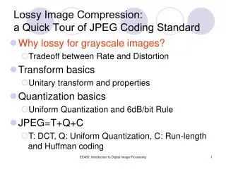
Lossy Image Compression:a Quick Tour of JPEG Coding Standard • Why lossy for grayscale images? • Tradeoff between Rate and Distortion • Transform basics • Unitary transform and properties • Quantization basics • Uniform Quantization and 6dB/bit Rule • JPEG=T+Q+C • T: DCT, Q: Uniform Quantization, C: Run-length and Huffman coding EE465: Introduction to Digital Image Processing
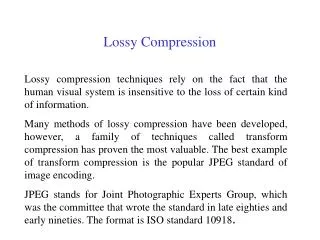
Why Lossy? • In most applications related to consumer electronics, lossless compression is not necessary • What we care is the subjective quality of the decoded image, not those intensity values • With the relaxation, it is possible to achieve a higher compression ratio (CR) • For photographic images, CR is usually below 2 for lossless, but can reach over 10 for lossy EE465: Introduction to Digital Image Processing
A Simple Experiment Bit-plane representation A=a0+a12+a222+ … … +a727 Least Significant Bit (LSB) Most Significant Bit (MSB) Example A=129 a0a1a2 …a7=10000001 a0a1a2 …a7=00110011A=4+8+64+128=204 EE465: Introduction to Digital Image Processing
A Simple Experiment (Con’t) • How will the reduction of gray-level resolution affect the image quality? • Test 1: make all pixels even numbers (i.e., knock down a0 to be zero) • Test 2: make all pixels multiples of 4 (i.e., knock down a0,a1 to be zeros) • Test 3: make all pixels multiples of 4 (i.e., knock down a0,a1,a2 to be zeros) EE465: Introduction to Digital Image Processing
Experiment Results Test 1 original Test 3 Test 2 EE465: Introduction to Digital Image Processing
How to Measure Image Quality? • Subjective • Evaluated by human observers • Do not require the original copy as a reference • Reliable, accurate yet impractical • Objective • Easy to operate (automatic) • Often requires the original copy as the reference (measures fidelity rather than quality) • Works better if taking HVS model into account EE465: Introduction to Digital Image Processing
Objective Quality Measures • Mean Square Error (MSE) • Peak Signal-to-Noise-Ratio (PSNR) original decoded Question: Can you think of a counter-example to prove objective measure is not consistent with subjective evaluation? EE465: Introduction to Digital Image Processing
Answer Shifted (MSE=337.8) Original cameraman image By shifting the last row of the image to become the first row, we affect little on subjective quality but the measured MSE is large EE465: Introduction to Digital Image Processing
Overview of JPEG Lossy Compression C T Q Flow-chart diagram of DCT-based coding algorithm specified by Joint Photographic Expert Group (JPEG) EE465: Introduction to Digital Image Processing
Lossy Image Compression:a Quick Tour of JPEG Coding Standard • Why lossy for grayscale images? • Tradeoff between Rate and Distortion • Transform basics • Unitary transform and properties • Quantization basics • Uniform Quantization and 6dB/bit Rule • JPEG=T+Q+C • T: DCT, Q: Uniform Quantization, C: Run-length and Huffman coding EE465: Introduction to Digital Image Processing
An Example of 1D Transform with Two Variables x2 y2 y1 (1,1) (1.414,0) x1 Transform matrix EE465: Introduction to Digital Image Processing
Generalization into N Variables forward transform basis vectors (column vectors of transform matrix) EE465: Introduction to Digital Image Processing
Decorrelating Property of Transform x2 y1 y2 x1 x1 and x2 are highly correlated y1 and y2 are less correlated p(x1x2) p(x1)p(x2) p(y1y2) p(y1)p(y2) EE465: Introduction to Digital Image Processing
Transform=Change of Coordinates • Intuitively speaking, transform plays the role of facilitating the source modeling • Due to the decorrelating property of transform, it is easier to model transform coefficients (Y) instead of pixel values (X) • An appropriate choice of transform (transform matrix A) depends on the source statistics P(X) • We will only consider the class of transforms corresponding to unitary matrices EE465: Introduction to Digital Image Processing
Unitary Matrix and 1D Unitary Transform Definition conjugate transpose A matrix A is called unitary if A-1=A*T When the transform matrix A is unitary, the defined transform is called unitary transform Example For a real matrix A, it is unitary if A-1=AT EE465: Introduction to Digital Image Processing
Inverse of Unitary Transform For a unitary transform, its inverse is defined by Inverse Transform basis vectors corresponding to inverse transform EE465: Introduction to Digital Image Processing
Properties of Unitary Transform • Energy compaction: only few transform coefficients have large magnitude • Such property is related to the decorrelating role of unitary transform • Energy conservation: unitary transform preserves the 2-norm of input vectors • Such property essentially comes from the fact that rotating coordinates does not affect Euclidean distance EE465: Introduction to Digital Image Processing
Energy Compaction Example Hadamard matrix significant insignificant EE465: Introduction to Digital Image Processing
Energy Conservation* A is unitary Proof EE465: Introduction to Digital Image Processing
Numerical Example Check: EE465: Introduction to Digital Image Processing
Implication of Energy Conservation Q T T-1 A is unitary EE465: Introduction to Digital Image Processing
Summary of 1D Unitary Transform Unitary matrix: A-1=A*T Unitary transform: A unitary Properties of 1D unitary transform Energy compaction: most of transform coefficients yi are small Energy conservation: quantization can be directly performed to transform coefficients EE465: Introduction to Digital Image Processing
From 1D to 2D Do N 1D transforms in parallel EE465: Introduction to Digital Image Processing
Definition of 2D Transform 2D forward transform 1D column transform 1D row transform EE465: Introduction to Digital Image Processing
2D Transform=Two Sequential 1D Transforms (left matrix multiplication first) column transform row transform row transform (right matrix multiplication first) column transform Conclusion: 2D separable transform can be decomposed into two sequential The ordering of 1D transforms does not matter EE465: Introduction to Digital Image Processing
Energy Compaction Property of 2D Unitary Transform Example A coefficient is called significant if its magnitude is above a pre-selected threshold th insignificant coefficients (th=64) EE465: Introduction to Digital Image Processing
Energy Conservation Property of 2D Unitary Transform 2-norm of a matrix X A unitary Example: You are asked to prove such property in your homework EE465: Introduction to Digital Image Processing
Implication of Energy Conservation Q T T-1 Similar to 1D case, quantization noise in the transform domain has the same energy as that in the spatial domain EE465: Introduction to Digital Image Processing
Important 2D Unitary Transforms • Discrete Fourier Transform • Widely used in non-coding applications (frequency-domain approaches) • Discrete Cosine Transform • Used in JPEG standard • Hadamard Transform • All entries are 1 • N=2: Haar Transform (simplest wavelet transform for multi-resolution analysis) EE465: Introduction to Digital Image Processing
Discrete Cosine Transform EE465: Introduction to Digital Image Processing
1D DCT forward transform inverse transform Properties Real and orthogonal • excellent energy compaction property DCT is NOT the real part of DFT Fact The real and imaginary parts of DFT are generally not orthogonal matrices fast implementation available: O(Nlog2N) EE465: Introduction to Digital Image Processing
2D DCT Its DCT coefficients Y (2451 significant coefficients, th=64) Original cameraman image X Notice the excellent energy compaction property of DCT EE465: Introduction to Digital Image Processing
Summary of 2D Unitary Transform • Unitary matrix: A-1=A*T • Unitary transform: A unitary • Properties of 2D unitary transform • Energy compaction: most of transform coefficients yi are small • Energy conservation: quantization can be directly performed to transform coefficients EE465: Introduction to Digital Image Processing
Lossy Image Compression:a Quick Tour of JPEG Coding Standard • Why lossy for grayscale images? • Tradeoff between Rate and Distortion • Transform basics • Unitary transform and properties • Quantization basics • Uniform Quantization and 6dB/bit Rule • JPEG=T+Q+C • T: DCT, Q: Uniform Quantization, C: Run-length and Huffman coding EE465: Introduction to Digital Image Processing
What is Quantization? • In Physics • To limit the possible values of a magnitude or quantity to a discrete set of values by quantum mechanical rules • In image compression • To limit the possible values of a pixel value or a transform coefficient to a discrete set of values by information theoretic rules EE465: Introduction to Digital Image Processing
Examples • Unlike entropy, we encounter it everyday (so it is not a monster) • Continuous to discrete • a quarter of milk, two gallons of gas, normal temperature is 98.6F, my height is 5 foot 9 inches • Discrete to discrete • Round your tax return to integers • The mileage of my car is about 55K. EE465: Introduction to Digital Image Processing
A Game Played with Bits • Precision is finite: the more precise, the more bits you need (to resolve the uncertainty) • Keep a card in secret and ask your partner to guess. He/she can only ask Yes/No questions: is it bigger than 7? Is it less than 4? ... • However, not every bit has the same impact • How much did you pay for your car? (two thousands vs. $2016.78) EE465: Introduction to Digital Image Processing
Scalar vs. Vector Quantization • We only consider the scalar quantization (SQ) in this course • Even for a sequence of values, we will process (quantize) each sample independently • Vector quantization (VQ) is the extension of SQ into high-dimensional space • Widely used in speech compression, but not for image compression EE465: Introduction to Digital Image Processing
^ ^ x x Definition of (Scalar) Quantization original value quantization index quantized value f f -1 sS x Quantizer Q x f finds the closest (in terms of Euclidean distance) approximation of x from a codebook C (a collection of codewords) and assign its index to s; f-1 operates like a table look-up to return the corresponding codeword EE465: Introduction to Digital Image Processing
^ x Numerical Example (I) C={-1,0,1} S={1,2,3} xR 1 2 3 -1 1 0 red: codewords green: index in C Three codewords 1 -0.5 x 0.5 -1 EE465: Introduction to Digital Image Processing
^ x Numerical Example (II) x{0,1,…,255} C={8,24,40,56,72,…,248} S={1,2,3,…,16} 16 1 2 3 ... 248 8 40 ... 24 red: codewords green: index in C sixteen codewords (note that the scales are different) 40 24 8 x floor operation 16 32 EE465: Introduction to Digital Image Processing
^ x Numerical Example (III) 232 216 232 232 216 200 216 40 56 56 72 40 136 104 88 24 225 222 235 228 220 206 209 44 49 56 64 42 128 106 94 27 Q x Notes For scalar quantization, each sample is quantized independently Quantization is irreversible EE465: Introduction to Digital Image Processing
Uniform Quantization for Uniform Distribution Uniform Quantization A scalar quantization is called uniform quantization (UQ) if all its codewords are uniformly distributed (equally-distanced) Example (quantization stepsize=16) 248 8 40 ... 24 Uniform Distribution denoted by U[-A,A] f(x) 1/2A x -A A EE465: Introduction to Digital Image Processing
Quantization Noise of UQ A -A f(e) 1/ e - /2 /2 Quantization noise of UQ on uniform distribution is also uniformly distributed Recall Variance of U[- /2, /2] is EE465: Introduction to Digital Image Processing
6dB/bit Rule Signal: X ~ U[-A,A] Noise: e ~ U[- /2, /2] Choose N=2n (n-bit) codewords for X (quantization stepsize) N=2n EE465: Introduction to Digital Image Processing
Lossy Image Compression:a Quick Tour of JPEG Coding Standard • Why lossy for grayscale images? • Tradeoff between Rate and Distortion • Transform basics • Unitary transform and properties • Quantization basics • Uniform Quantization and 6dB/bit Rule • JPEG=T+Q+C • T: DCT, Q: Uniform Quantization, C: Run-length and Huffman coding EE465: Introduction to Digital Image Processing
JPEG Coding Algorithm Overview EE465: Introduction to Digital Image Processing
Transform Coding of Images • Why not transform the whole image together? • Require a large memory to store transform matrix • It is not a good idea for compression due to spatially varying statistics within an image • Idea of partitioning an image into blocks • Each block is viewed as a smaller-image and processed independently • It is not a magic, but a compromise EE465: Introduction to Digital Image Processing
Block-based DCT Example I J note that white lines are artificially added to the border of each 8-by-8 block to denote that each block is processed independently EE465: Introduction to Digital Image Processing
Boundary Padding Example 12 13 14 15 16 17 18 19 12 13 14 15 16 17 18 19 12 13 14 15 16 17 18 19 12 13 14 15 16 17 18 19 padded regions When the width/height of an image is not the multiple of 8, the boundary is artificially padded with repeated columns/rows to make them multiple of 8 EE465: Introduction to Digital Image Processing