Download
1 / 27
270 likes | 356 Vues
Stratosphere-Troposhere Coupling in Dynamical Seasonal Predictions. Bo Christiansen. Danish Meteorological Institute. Motivation. Opinion of some dynamical forecasters:

E N D
Stratosphere-Troposhere Coupling in Dynamical Seasonal Predictions BoChristiansen Danish Meteorological Institute
Motivation Opinion of some dynamical forecasters: Stratosphere-troposphere coupling is not important, the stratospheric signal is just an imprint of what is going on in the troposphere Stratosphere-troposphere coupling is already included in the models Let us forget about the stratosphere and increase the horizontal resolution
Layout of the talk: What kind of behaviour should we expect? Simple statistical forcasts based only on observations. Dynamical model has to do better than that. Why should we expect the stratosphere-troposphere coupling to be included in dynamical models? Some results from a dynamical seasonal prediction system
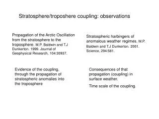
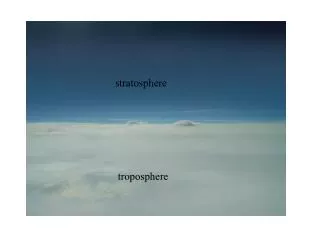
Downward propagation of zonal mean zonal wind in ERA40. Annual cycle and timescales faster than 30 days are removed. Watch the movie at www.dmi.dk/solar-terrestrial/staff/boc/homepage.shtml
My choice of zonal index: the zonal mean zonal wind a 60 N • Advantages compared to EOF based indices: • simple physical meaning • easy to calculate • archived for most GCM experiments • no risk of spurious modes due to noise and no mode mixing At the surface it is strongly correlated with the AO/`NAO In the stratosphere it is strongly correlated with the strenghth of the vortex
Predicting surface zonal wind Forecast of daily values 70 hPa Forecast skill as function of lead time T for different vertical levels of the predictor. 10 hPa surface Purple curve shows forecast when wind at surface and at 70 hPa are used as predictors simultaneously Forecast of 14 days means 70 hPa 10 hPa surface Only winter, DJF
Predicting surface zonal wind The forecast skill as function of lead time and the vertical level of the predictor. Shaded regions are where correlations are significantly different from zero at 99 and 95 % levels. Calculated by Monte-Carlo approach assuming normality and observed temporal structure. Daily values are predicted. Winter season.
The forecast skill as function of lead time and the time over which the predictand is averaged. The level of the predictor is 70 hPa. The forecast skill as function of lead time and the strength of the predictor. 14 days means are forecasted.
Comparison with dynamical forecast. 51 events from the ECMWF ensemble seasonal prediction system 2 Model Model+70 hPa 70 hPa 70 hPa, 51 events surface Predictand is surface wind at 60 N, Daily values are forecasted.
Downward propagation is robust and ubiquitous Minimal model Holton Mass model Perp. Jan. GCM Full GCM Observations Zonal wind at 60 N
Vertical component of EP-flux at 60 N Vertical component of EP-flux at 100 hPa Zonal mean wind at 60 N
Covariance between zonal mean wind at 10 hPa, 60 N and components in the balance equation for zonal monentum. Lag (days)
height Radiative equilibrium wind The basic mechanism
A minimal model Coriolis term Zonal wind trend Wave coupling 1-dimensional: Simple resistance: Nonlinear coupling (Charney-Drazin):
How much does the stratosphere control? 5 different transient perturbations in 10 different layers, 8 different initial conditions ARPEGE GCM, perpetual Januarry Christiansen, QJRMS., 129, 2003.
Experiments with constant troposphere show that vacillations can exist without growth of disturbances
Errors grow like a power-law, not exponential Not like deterministic chaos in low dimensional systems. However, systems with many degrees of freedom can show power-law growthof perturbations as shown by Lorenz (1969).
There are some reasons to believe that dynamical forecast models may already include the stratsphere-troposphere coupling: • The coupling is present in models of different complexities • At least part of the coupling can be explained by a simple • mechanism (which unlike the QBO depends on large-scale waves) • The coupling is well represented in the ARPEGE GCM Perhaps the stratosphere is only passively responding to tropospheric processes, perturbations may develop independent of the downward propagation
ECMWFs dynamical ensemble seasonal prediction system • Hindcasts with 11 ensemble members1981-2005 • Model has 62 vertical levels with top at 5 hPa • But: Only archived at 10 levels .. 200, 50, 10 hPa • ERA40 has .. 200, 150, 100, 70, 50, 30, 20, 10 hPa • Initial conditions based on ERA40 for 1981-2001 and • operational analysis for 2002-2005 • Model started the first day of every months, giving 3x25 • different DJF events
Ensembe mean One example of the ensemble forecast Target
One example of ensemble mean forecast Forecast Target Target reduced to 10 layers Forecast - Target
Lagged correlations between U at10 hPa and U at other levels ERA40, all data Shaded regions are where correlations are significantly different from zero at 99 and 95 % levels. Calculated by a t-test assuming normality and independent predictions
Model Observations
Forecast skill at the surface: Correlations between forecast and target Dynamical Model Stat. model
Conclusions • Downward propagation is ubiquitous: found in observations and models of different complexity • Downward propagation driven by waves from the troposphere and the two-way interaction between mean flow and waves is important • Dynamical seasonal prediction model does include stratosphere-troposphere coupling • But this coupling is too strong compared to observations • Dynamical prediction model strongly overestimates the decorrelation time in the stratosphere. Also somewhat overestimated in the troposphere. • Dynamical prediction model has more skill in the stratosphere compared to the statistical model for lead times up to 50 days.