Download
1 / 44
440 likes | 567 Vues
Multi-model ensemble predictions on seasonal timescales. Tim Stockdale European Centre for Medium-Range Weather Forecasts (Some material from Antje Weisheimer ). Structure of the lecture. The multi-model concept Example: results from DEMETER

E N D
Multi-model ensemble predictionson seasonal timescales Tim Stockdale European Centre for Medium-Range Weather Forecasts (Some material from Antje Weisheimer)
Structure of the lecture The multi-model concept Example: results from DEMETER Under which conditions can a multi-model ensemble outperform the best single-model? EUROSIP – operational multi-model forecasts
Model error • By model error we mean problems, inadequacies and imperfections with the model formulation and its numerical implementation. • This model error causes integrations of the model to produce results which are unrealistic in various ways; e.g. the model climate (mean, variability, features) may be unrealistic. • The imperfections in the model also contribute to errors in any seasonal forecast produced by the model. This contribution we define as the model forecast error. We do not know its value in any particular case, but may try to estimate its statistical properties.
Multi-model ensemble • Different coupled GCMs have different model errors • There may be lots of common errors, too. • So let’s take an ‘ensemble’ of model forecasts: • The mean of the ensemble should be better, because at least some of the model forecast errorswill be averaged out • The ‘spread’ of the ensemble should be better, since we are sampling some of the uncertainty • An ensemble of forecast values or of models?
Multi-model ensemble of forecast values • What would an ‘ideal’ multi-model system look like? • Assume fairly large number of models (10 or more) • Assume models have roughly equal levels of forecast error • Assume that model forecast errors are uncorrelated • Assume that each model has its own mean bias removed • A priori, for each forecast, we consider each of the models’ forecasts equally likely [in a Bayesian sense – in reality, all the model pdfs will be wrong] • A posteriori, this is no longer the case: model forecasts near the centre of the multi-model distribution have higher likelihood • Different from a single model ensemble with perturbed ic’s. • Multi-model ensemble distribution is NOT a pdf
Time 1 Time 2 Error in ensemble mean = σe/ √n
Non-ideal case • Model forecast errors are not independent • Dependence will reduce degrees of freedom, hence the effective n; this will increase uncertainty • In some cases, reduction in n could be drastic • Model forecast errors may have different amplitudes • And we may not know which models are better • Initial condition error can be important • The foregoing analysis applies only to the ‘model error’ contribution to error variance • Initial condition error must be accounted for separately; it is less likely to be independent.
Multi-model ensemble is not a pdf Although we can choose to treat it as one if we want (and many people do).
Forecast process Forecast pdfshould be an appropriate interpretation of model ensemble, not an equivalence.
DEMETER – a worked example of multi-model seasonal forecasts
The DEMETER project multi-model of 7 coupled general circulation models • hindcast production period: 1958-2001 • 9-member IC ensembles for each model • ERA-40 initial conditions • SST and wind perturbations • 4 start dates per year: 1st of Feb, May, Aug, and Nov • 6 month hindcasts http://www.ecmwf.int/research/demeter/
Feb 87 May 87 Aug 87 Nov 87 Feb 88 ... The DEMETER project multi-model of 7 coupled general circulation models 7 models x 9 ensemble members 63-member multi-model ensemble = 1 hindcast Production for 1958-2001 = 44x4 = 176 hindcasts
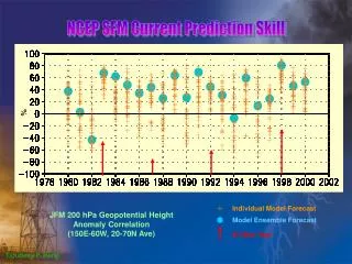
SST MSLP multi-model baseline model ranking DEMETER: multi-model vs single-model Relative ACC improvement of the multi-model compared to the single models for JJA from 1980-2001 (one month lead) Hagedorn et al. (2005) Anomaly Correlation Coefficients (ACC)
SST MSLP multi-model baseline model ranking DEMETER: multi-model vs single-model Relative improvement of the multi-model compared to the single models for JJA from 1980-2001 (one month lead) for different scores. Tropics Anomaly Correlation Coefficients (ACC), root mean square skill score (RMSSS), Ranked Probability Skill Score (RPSS) and ROC Skill Score (ROCSS) Hagedorn et al. (2005)
(1959-2001) single-model multi-model DEMETER: Brier score of multi-model vs single-model Brier skill score Hagedorn et al. (2005)
Resolution skill score Reliability skill score single-model single-model multi-model multi-model DEMETER: Brier score of multi-model vs single-model • improved reliability of the multi-model predictions • improved resolution of the multi-model predictions Hagedorn et al. (2005)
0.039 0.899 0.141 0.095 0.926 0.169 -0.001 0.877 0.123 0.039 0.899 0.140 0.204 0.990 0.213 0.047 0.893 0.153 0.065 0.918 0.147 -0.064 0.838 0.099 multi-model DEMETER: multi-model vs single-model BSS Rel-Sc Res-Sc Reliability diagrams (T2m > 0) 1-month lead, start date May, 1980 - 2001 Hagedorn et al. (2005)
DEMETER: impact of ensemble size • Is the multi-model skill improvement due to • increase in ensemble size? • using different sources of information? • An experiment with the ECMWF coupled model and 54 ensemble members to assess • impact of the ensemble size • impact of the number of models
0.170 0.959 0.211 0.222 0.994 0.227 Hagedorn et al. (2005) DEMETER: impact of ensemble size 1-month lead, start date May, 1987 - 1999 BSS Rel-Sc Res-Sc Reliability diagrams (T2m > 0) 1-month lead, start date May, 1987 - 1999 multi-model [54 members] single-model [54 members]
DEMETER: impact of number of models Multi-model realizations Single-model realizations
Under which conditions can a multi-model ensemble outperform the best single-model?
Where does the success of the multi-model come from? • Weigel, Liniger and Appenzeller (2008): • Toy model: Synthetic forecast generator for perfectly calibrated single model ensembles of any size and skill with prescribed ensemble underdispersion (or overconfidence) x: observation f(x): ensemble forecast a: average correlation coefficient between fi and x b: overconfidence parameter (b=0 well-dispersed ensemble)
Where does the success of the multi-model come from? Illustration of the toy model effect of correlation afor a well-dispersed ensemble(b=0) effect of overconfidence bfor a constant correlation(a=0.65) Weigel et al. (2008) Two examples of εβ
Where does the success of the multi-model come from? Multi-model ensemble can locally outperform the best member, but only if the single model ensembles are overconfident i.e. if model forecast error exists Two overconfident (b=0.7)single-model ensemblesa1, a2 Two well dispersed (b=0)single-model ensemblesa1, a2 RPSS skill matrix RPSSmulti-modelminusRPSSbest single model Weigel et al. (2008)
Where does the success of the multi-model come from? Multi-model combination reduces overconfidence, that is ensemble spread is widened while the average ensemble mean error is reduced • net gain in prediction skill over best model because probabilistic skill scores penalize overconfidence • even the addition of an objectively poor model can improve multi-model skill Weigel et al. (2008)
Where does the success of the multi-model come from? • Is multi-model better than “inflating” a single model ensemble to get a pdf? If so, why? • Generally yes. • “Inflation” applies to all forecasts. A multi-model system contains information on which cases are more trustworthy (high consensus) and which are less so. It really adds information. • As long as the additional models are not too poor compared to the best single model (or best subset).
EUROSIP multi-model ensemble • Fourmodels at ECMWF: • ECMWF – as described • Met Office – HADGEM model, Met Office ocean analyses • Météo-France – Météo-France model, Mercator ocean analyses • NCEP – CFSv2 • Unified system • Real-time since mid-2005 • All data in ECMWF operational archive • Common operational schedule (products released at 12Z on 15th) • Recent changes at Met Office have limited the system somewhat • See “EUROSIP User Guide” on web for details, and also the ECMWF Newsletter article (Issue No. 118, Winter 2008/09)
EUROSIP data • Individual model data archived in MARS • Daily and monthly means • Available to Member States for official duty use • Available for research and education • Multi-model data products • Created and archived in MARS • Available for dissemination, also for commercial customers • International support • WMO access to multi-model web products • Multi-model data supplied to EUROBRISA project in Brazil
Variance scaling • Robust implementation • Limit to maximum scaling (1.4) • Weakened upscaling for very large anomalies • Improves every individual model • Improves consistency between models • Improves accuracy of multi-model ensemble mean
Method for p.d.f. estimation (1) • Assume underlying normality • Calculate robust skill-weighted ensemble mean • Do not try a multivariate fit (very small number of data points) • Weights estimated ~1/(error variance). Would be optimal for independent errors – i.e., is conservative. • Then use 50% uniform weighting, 50% skill dependent • Comments: • Rank weighting also tried, but didn’t help. • QC term tried, using likelihood to downplay impact of outliers, but again didn’t help. Outliers are usually wrong, but not always. • Models usually agree reasonably well, and tweaks to weights have very little impact anyway.
Method for p.d.f. estimation (2) • Re-centre lower-weighted models • To give correct multi-model ensemble mean • Done so as to minimize disturbance to multi-model spread • Compare past ensemble and error variances • Use above method (cross-validated) to generate past ensembles • Unbiased estimates of multi-model ensemble variance and observed error variance • Scale forecast ensemble variance • 50% of variance is from the scaled climatological value, 50% from the scaled forecast value • Comments: • For multi-model, use of predicted spread gives better results • For single model, seems not to be so.
Method for p.d.f. estimation (3) • Estimate t distribution • Variance estimates are based on small samples, ~15 points • Need to use ‘t’ distribution to estimate resulting p.d.f. • Finite d.o.f. due to both number of years and ensemble size • Plot p.d.f. • Specified percentiles, or plume with 2%ile intervals • Or plot forecast values with calibrated mean and variance • Comments: • Can apply to single model or multi-model • Small ensemble size -> large width of p.d.f.
P.d.f. interpretation • P.d.f. based on past errors • The risk of a real-time forecast having a new category of error is not accounted for. E.g. Tambora volcanic eruption. • We plot 2% and 98%ile. Would not go beyond this in tails. • Risk of change in bias in real-time forecast relative to re-forecast. • Bayesian p.d.f. • Explicitly models uncertainty coming from errors in forecasting system • Two different systems will calculate different pdf’s – both are correct • Validation • Rank histograms show pdf’s are remarkably accurate (cross-validated) • Verifying different periods shows relative bias of different periods can distort pdf – sampling issue in our validation data.
ECMWF forecast: ENSO Past performance
EUROSIP forecast: ENSO Past performance
Multi-model Single model
Summary • Multi-model ensemble forecasting is a pragmatic and efficient method to filter out some of the model errors present in the individual ensemble forecasts and enhance ensemble spread • Multi-model predictions yield, on average, more accurate predictions than any of the individual single-model ensembles (e.g., DEMETER) • The improvement is mainly due to more consistency and increased reliability and due to the reduced overconfidence from single-model ensembles • Still need better models!
References (I) • Doblas-Reyes, F.J., R. Hagedorn and T.N. Palmer, 2005: The rationale behind the success of multi-model ensembles in seasonal forecasting. Part II: Calibration and combination. Tellus, 57A, 234-252. • Hagedorn, R., F.J. Doblas-Reyes and T.N. Palmer, 2005: The rationale behind the success of multi-model ensembles in seasonal forecasting. Part I: Basic concept. Tellus, 57A, 219-233. • Joliffe, I.T. and D.B. Stephenson (Ed.), 2003: Forecast verification: A practitioner’s guide in atmospheric science. Wiley New York, 240pp. • Judd, K., L.A. Smith and A. Weisheimer, 2007: How good is an ensemble at capturing truth? : Bounding boxes. Quart. J. R. Meteorol. Soc.,133, 1309-1325. • Murphy, A.H., 1993: What is a good forecast? An essay on the nature of goodness in weather forecasting. Wea. Forecasting, 8, 281-293. • Palmer, T.N. et al, 2004: Development of a European multi-model ensemble system for seasonal to inter-annual prediction (DEMETER). Bull. Am. Meteorol. Soc.,85, 853-872.
References (II) • Palmer, T.N., F. Doblas-Reyes, A. Weisheimer and M. Rodwell, 2008: Towards seamless prediction: Calibration of Climate-Change Projections using Seasonal Forecasts. Bull. Am. Meteorol. Soc.,89, 459-470. • Vitart, F., 2006: Seasonal forecasting of tropical storm frequency using a multi-model ensemble. Q.J.R.Meteorol.Soc., 132, 647-666. • Vitart, F. M. Huddleston, M. Deque, D. Peake, T.N. Palmer, T.N. Stockdale, M. Davey, S. Ineson and A. Weisheimer, 2007: Dynamically-based seasonal forecasts of Atlantic tropical-storm activity. Geophys. Res. Lett., 34, L16815, doi:10.1029/2007GL030740. • Weigel, A.P., M.A. Liniger and C. Appenzeller, 2008: Can multi-model combination really enhance the prediction skill of probabilistic ensemble forecasts? Q.J.R.Meteorol. Soc.,134, 241-260. • Weisheimer, A., L.A. Smith and K. Judd, 2005: A new view of seasonal forecast skill: Bounding boxes from the DEMETER ensemble forecasts. Tellus, 57A, 265-279. • Weisheimer, A. and T.N. Palmer, 2005: Changing frequency of occurrence of extreme seasonal temperatures under global warming. Geophys. Res. Lett., 32, L20721, doi:10.1029/2005GL023365. Special issue in Tellus (2005), Vol. 57A on DEMETER