Download

1 / 29
290 likes | 474 Vues
Lecture 10 Secondary Structure Prediction. Bioinformatics Center IBIVU. Protein primary structure. 20 amino acid types A generic residue Peptide bond. SARS Protein From Staphylococcus Aureus. 1 MKYNNHDKIR DFIIIEAYMF RFKKKVKPEV 31 DMTIKEFILL TYLFHQQENT LPFKKIVSDL

E N D
Lecture 10Secondary Structure Prediction Bioinformatics Center IBIVU
Protein primary structure 20 amino acid types A generic residue Peptide bond SARS Protein From Staphylococcus Aureus 1MKYNNHDKIR DFIIIEAYMF RFKKKVKPEV 31 DMTIKEFILL TYLFHQQENTLPFKKIVSDL 61 CYKQSDLVQH IKVLVKHSYI SKVRSKIDER 91 NTYISISEEQ REKIAERVTL FDQIIKQFNL 121 ADQSESQMIP KDSKEFLNLM MYTMYFKNII 151 KKHLTLSFVE FTILAIITSQ NKNIVLLKDL 181 IETIHHKYPQ TVRALNNLKKQGYLIKERST 211 EDERKILIHM DDAQQDHAEQ LLAQVNQLLA 241 DKDHLHLVFE
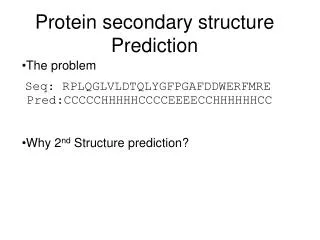
Protein secondary structure Alpha-helix Beta strands/sheet SARS Protein From Staphylococcus Aureus 1 MKYNNHDKIR DFIIIEAYMF RFKKKVKPEV DMTIKEFILL TYLFHQQENT SHHH HHHHHHHHHH HHHHHHTTT SS HHHHHHH HHHHS S SE 51 LPFKKIVSDL CYKQSDLVQH IKVLVKHSYI SKVRSKIDER NTYISISEEQ EEHHHHHHHS SS GGGTHHH HHHHHHTTS EEEE SSSTT EEEE HHH 101 REKIAERVTL FDQIIKQFNL ADQSESQMIP KDSKEFLNLM MYTMYFKNII HHHHHHHHHH HHHHHHHHHH HTT SS S SHHHHHHHH HHHHHHHHHH 151 KKHLTLSFVE FTILAIITSQ NKNIVLLKDL IETIHHKYPQ TVRALNNLKK HHH SS HHH HHHHHHHHTT TT EEHHHH HHHSSS HHH HHHHHHHHHH 201 QGYLIKERST EDERKILIHM DDAQQDHAEQ LLAQVNQLLA DKDHLHLVFE HTSSEEEE S SSTT EEEE HHHHHHHHH HHHHHHHHTS SS TT SS
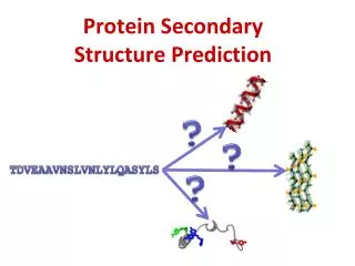
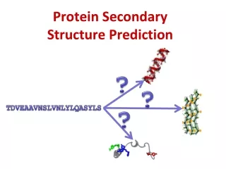
Protein secondary structure • Why bother predicting them? • Framework model of protein folding, collapse secondary structures • Fold prediction by comparing to database of known structures • Can be used as information to predict function
Why predict when you can have the real thing? UniProt Release 1.3 (02/2004) consists of:Swiss-Prot Release : 144731 protein sequencesTrEMBL Release : 1017041 protein sequences PDB structures : : 24358 protein structures Primary structure Secondary structure Tertiary structure Quaternary structure Function
What we need to do • Train a method on a diverse set of proteins of known structure • Test the method on a test set separate from our training set • Assess our results in a useful way against a standard of truth • Compare to already existing methods using the same assessment
How to develop a method Other method(s) prediction Test set of T<<N sequences with known structure Database of N sequences with known structure Standard of truth Assessment method(s) Method Prediction Training set of K<N sequences with known structure Trained Method
Some key features ALPHA-HELIX: Hydrophobic-hydrophilic residue periodicity patterns BETA-STRAND: Edge and buried strands, hydrophobic-hydrophilic residue periodicity patterns OTHER: Loop regions contain a high proportion of small polar residues like alanine, glycine, serine and threonine. The abundance of glycine is due to its flexibility and proline for entropic reasons relating to the observed rigidity in its kinking the main-chain. As proline residues kink the main-chain in an incompatible way for helices and strands, they are normally not observed in these two structures, although they can occur in the N-terminal two positions of a-helices. Edge Buried
Burried and Edge strands Parallel -sheet Anti-parallel -sheet
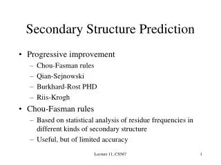
History (1) Using computers in predicting protein secondary has its onset 30 ago (Nagano (1973) J. Mol. Biol., 75, 401) on single sequences. The accuracy of the computational methods devised early-on was in the range 50-56% (Q3). The highest accuracy was achieved by Lim with a Q3 of 56% (Lim, V. I. (1974) J. Mol. Biol., 88, 857). The most widely used method was that of Chou-Fasman (Chou, P. Y. , Fasman, G. D. (1974) Biochemistry, 13, 211). Random prediction would yield about 40% (Q3) correctness given the observed distribution of the three states H, E and C in globular proteins (with generally about 30% helix, 20% strand and 50% coil).
History (2) Nagano 1973 – Interactions of residues in a window of 6. The interactions were linearly combined to calculate interacting residue propensities for each SSE type (H, E or C) over 95 crystallographically determined protein tertiary structures. Lim 1974 – Predictions are based on a set of complicated stereochemical prediction rules for a-helices and b-sheets based on their observed frequencies in globular proteins. Chou-Fasman 1974 - Predictions are based on differences in residue type composition for three states of secondary structure: a-helix, b-strand and turn (i.e., neither a-helix nor b-strand). Neighbouring residues were checked for helices and strands and predicted types were selected according to the higher scoring preference and extended as long as unobserved residues were not detected (e.g. proline) and the scores remained high.
GOR: the older standard The GOR method (version IV) was reported by the authors to perform single sequence prediction accuracy with an accuracy of 64.4% as assessed through jackknife testing over a database of 267 proteins with known structure. (Garnier, J. G., Gibrat, J.-F., , Robson, B. (1996) In: Methods in Enzymology (Doolittle, R. F., Ed.) Vol. 266, pp. 540-53.) The GOR method relies on the frequencies observed for residues in a 17- residue window (i.e. eight residues N-terminal and eight C-terminal of the central window position) for each of the three structural states.
How do secondary structure prediction methods work? • They often use a window approach to include a local stretch of amino acids around a considered sequence position in predicting the secondary structure state of that position • The next slides provide basic explanations of the window approach (for the GOR method as an example) and two basic techniques to train a method and predict SSEs: k-nearest neighbour and neural nets
Sliding window Central residue Sliding window Sequence of known structure H H H E E E E • The frequencies of the residues in the window are converted to probabilities of observing a SS type • The GOR method uses three 17*20 windows for predicting helix, strand and coil; where 17 is the window length and 20 the number of a.a. types • At each position, the highest probability (helix, strand or coil) is taken. A constant window of n residues long slides along sequence
K-nearest neighbour Sequence fragments from database of known structures (exemplars) Sliding window Compare window with exemplars Qseq Central residue Get k most similar exemplars PSS HHE
Neural nets Sequence database of known structures Sliding window Qseq Central residue Neural Network The weights are adjusted according to the model used to handle the input data.
Training an NN: • Forward pass: • the outputs are calculated and the error at the output units calculated. • Backward pass: • The output unit error is used to alter weights on the output units. Then the error at the hidden nodes is calculated (by back-propagating the error at the output units through the weights), and the weights on the hidden nodes altered using these values. • For each data pair to be learned a forward pass and backwards pass is performed. This is repeated over and over again until the error is at a low enough level (or we give up). Neural nets Y = 1 / (1+ exp(-k.(Σ Win * Xin)), where Win is weight and Xinis input The graph shows the output for k=0.5, 1, and 10, as the activation varies from -10 to 10.
Example of widely used neural net method:PHD, PHDpsi, PROFsec • The three above names refer to the same basic technique and come from the same laboratory (Rost’s lab at Columbia, NYC) • Three neural networks: • A 13 residue window slides over the alignment and produces 3-state raw secondary structure predictions. • A 17-residue window filters the output of network 1. The output of the second network then comprises for each alignment position three adjusted state probabilities. This post-processing step for the raw predictions of the first network is aimed at correcting unfeasible predictions and would, for example, change (HHHEEHH) into (HHHHHHH). • A network for a so-called jury decision over a set of independently trained networks 1 and 2 (extra predictions to correct for training biases). The predictions obtained by the jury network undergo a final simple filtering step to delete predicted helices of one or two residues and changing those into coil.
Multiple Sequence Alignments are the superior input to a secondary structure prediction method Multiple sequence alignment: three or more sequences that are aligned so that overall the greatest number of similar characters are matched in the same column of the alignment. • Enables detection of: • Regionsof high mutation rates over evolutionary time. • Evolutionary conservation. • Regions or domains that are critical tofunctionality. • Sequence changes that cause a change in functionality. Modern SS prediction methods all use Multiple Sequence Alignments (compared to single sequence prediction >10% better)
Rules of thumb when looking at a multiple alignment (MA) • Hydrophobic residues are internal • Gly (Thr, Ser) in loops • MA: hydrophobic block -> internal -strand • MA: alternating (1-1) hydrophobic/hydrophilic => edge -strand • MA: alternating 2-2 (or 3-1) periodicity => -helix • MA: gaps in loops • MA: Conserved column => functional? => active site
Rules of thumb when looking at a multiple alignment (MA) • Active site residues are together in 3D structure • MA: ‘inconsistent’ alignment columns and alignment match errors! • Helices often cover up core of strands • Helices less extended than strands => more residues to cross protein • -- motif is right-handed in >95% of cases (with parallel strands) • Secondary structures have local anomalies, e.g. -bulges
A stepwise hierarchy Thesebasically are local alignment techniques to collect homologous sequences from a database so a multiple alignment containing the query sequence can be made (we will talk about these methods later) • Sequence database searching • PSI-BLAST, SAM-T2K • 2) Multiple sequence alignment of selected sequences • PSSMs, HMM models, MSAs • 3) Secondary structure prediction of query sequences • based on the generated MSAs • Single methods: PHD, PROFsec, PSIPred, SSPro, JNET, YASPIN • consensus
Sequence database Sequence database PSI-BLAST SAM-T2K The current picture Single sequence Step 1: Database sequence search Step 2: MSA Check file PSSM Homologous sequences HMM model MSA method MSA Step 3: SS Prediction Trained machine-learning Algorithm(s) Secondary structure prediction
Jackknife test A jackknife test is a test scenario for prediction methods that need to be tuned using a training database. Its simplest form: For a database containing N sequences with known tertiary (and hence secondary) structure, a prediction is made for one test sequence after training the method on the remaining training database containing the N-1 remaining sequences (one-at-a-time jackknife testing). A complete jackknife test would involve N such predictions. If N is large enough, meaningful statistics can be derived from the observed performance. For example, the mean prediction accuracy and associated standard deviation give a good indication of the sustained performance of the method tested. If this is computationally too expensive, the database can be split in larger groups, which are then jackknifed.
Jackknifing a method For jackknife test: T=1 Other method(s) prediction Test set of T<<N sequences with known structure Database of N sequences with known structure Standard of truth Assessment method(s) Method Prediction Training set of K<N sequences with known structure Trained Method For full jackknife test: Repeat process N times and average prediction scores For jackknife test: K=N-1
Standards of truth What is a standard of truth? - a structurally derived secondary structure assignment (using a 3D structure from the PDB) Why do we need one? - it dictates how accurate our prediction is How do we get it? - methods use hydrogen-bonding patterns along the main-chain to define the Secondary Structure Elements (SSEs).
Some examples of programs that assign secondary structures in 3D structures • DSSP (Kabsch and Sander, 1983) – most popular • STRIDE (Frishman and Argos, 1995) • DEFINE (Richards and Kundrot, 1988) • Annotation: • Helix: 3/10-helix (G), -helix (H), -helix (I) • Strand: -strand (E), -bulge (B) • Turn: H-bonded turn (T), bend (S) • Rest: Coil (“ “)
Assessing a prediction How do we decide how good a prediction is? • Qn : the number of correctly predicted n SSEstates over the total number of predicted states • Segment OVerlap (SOV): the number of correctly predicted n SSE states over the total number of predictions with higher penalties for core segment regions (Zemla et al, 1999) • Matthews Correlation Coefficients (MCC): the number of correctly predicted n SSE states over the total number of predictions taking into account how many prediction errors were made for each state
Single vs. Consensus predictions The current standard ~1% better on average Predictions from different methods H H H E E E E C E Max observations are kept as correct