Download
1 / 30
500 likes | 889 Vues
The Onsager solution of the 2d Ising model (continued). Summary of first part. Notation:. Fourier, of course. By fermionization V becomes an infinite interacting 1d periodic Fermi system . Jean Baptiste Joseph Fourier.

E N D
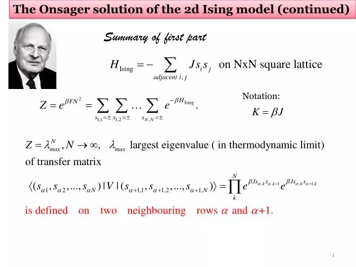
The Onsager solution of the 2d Ising model (continued) Summary of first part Notation:
Fourier, of course By fermionization V becomes an infinite interacting 1d periodic Fermi system. Jean Baptiste Joseph Fourier a second-quantization operator with the structure of an exponential. Thisfictitioussystemwillcontain an unspecifiednumber of interactingparticlesand we must seek the largesteigenvalue.
different q are decoupled and the problem reduces to diagonalizing End of summary of first part We shall find simultaneous eigenvectors of Simultanouseigenstates of those operators are eigenstates ofVq. In stateslabelled by q onefindseither 0 or 1 particles, and one can create in both q and –q butonly once. The dimension of the Hilbertspaceisjust 4. 3
Diagonalization of Vq In states labelled by q one finds either 0 or 1 particles, and one can create in both q and –q but only once. Whatis the Hilbertspace? 4 basisvectors per q The average over the pair state is obtained by setting occupation numbers =1.
By hand this product is tedious. Fullsimplify on Mathematica yelds:
From one can work out, recalling that V is hermitean and eigenvalues must be real: 9
The free energy per spin is The solution is a bit implicit, but complete !
Actually, one can obtain (see Huang page 386) the slightly more explicit expression Temperature dependence of energy per spin Temperature dependence of specific heat
Phase transition Temperature dependence of spontaneous magnetization (Yang’s calculation, not Onsager’s, where H=0),see Huang page 391 14
Monte Carlo simulations The exactsolutionoffers a unique benchmark for computer simulations by a Metropolisalgorithm. Lattices of up and down spins are producedby random number generation using an algorithmbased on importancesampling. Given a lattice one spin isturned and the new energyevaluated. The new lattice isacceptedif the energyisnottoo high. Thenaverages are computed.
(Weiss theory) (Weiss theory) 20
The Ising model including H is soluble if we assume N>>1 nearest neighbours (many dimensions or very long-range interaction): we must divide interaction by N to have a finite answer for large N. So we take: Wecalculate Z exactly via the Hubbard-Stratonovichtransformation
the minimum condition is With Evaluationof Z by the steepestdescentmethod
Recall the Weiss mean field theory (1907) Exchange field PIERRE-ERNEST WEISS born March 25, 1865, Mulhouse, France. died Oct. 24, 1940, Lyon, France. The behavior of an Ising model on a fully connected graph may be completely understood by mean field theory,because each site has a very large number of neighbors. Each spin interacts with all the others, Only the average number of + spins and − spins is important, since the fluctuations about this mean will be very small. Mean field = exact in infinite d
k>0 Mermin-Wagner theorem in Statistical Mechanics, = (Coleman theorem (1973) in QFT) In d=1 and d=2 continuous symmetries cannot be spontaneously broken at finite T in systems with sufficiently short ranged interactions. This does not apply to discrete symmetries (2d Ising model) Thinfilms do show phasetransitionsexperimentally, so perhapsthey are notreally2d. In additiontopologicaltransitions (no brokensymmetry) can occur in 2d. X-Y model and Kosterlitz-Thouless topological transition Vorticescanotoccur in 1d. Since KT deal with vorticeswedigress a littleaboutfluids. For a 2d fluidmoving with velocity u(x,y,t) in 2d the vorticityis
In polar coordinates with basis vectors consider a circular vortex If the densityisr, the kineticenergyof the vortexisfinite ifwe introduce twocutofflengths: size R of the fluid, and intermoleculardistance r0 In a similar way one can compute the energy of twovortices of opposite vorticityat a distance d and findthattheyattracteachother. Onefindsthat the interactionenergygrows with the distanceas Vortex and antivortexattracteachother and annihilate.
X-Y model and the KT transition Classicalspins confined in (x,y) plane in a 2d lattice; the oneat site j makes an angle qj with the x axis. The Hamiltonianis: In the groundstatesall spins are aligned in some direction, and every cos =1 Excitationsare vortices and monopoles. They are topological, thatis, they are likeholes in the system. I take figures from Mahan’sNutshell book
Above, the systemcreates free vortices Below, excitationsconsist of vortex-antivortexpairs. No symmetryisbroken in the transition.