Download
1 / 20
250 likes | 494 Vues
THE ISING PHASE IN THE J1-J2 MODEL. Valeria Lante and Alberto Parola. {. the model motivation phase diagram. OUTLINE :. introduction to the model our aim analytical approach numerical approach Conclusions the future. non linear sigma model. Lanczos exact diagonalizations.

E N D
THE ISING PHASE IN THE J1-J2 MODEL Valeria Lante and Alberto Parola
{ the model motivation phase diagram OUTLINE: introduction to the model our aim analytical approach numerical approach Conclusions the future non linear sigma model Lanczos exact diagonalizations
J1 J2 spin systems: symmetry breaking (magnetization) (no 1D for Mermin-Wagner theorem) T = 0 ? Can quantum fluctuations stabilize a disordered phase in spin systems at T=0 ? INTRODUCTION: What is the J1-J2model ? Why the J1-J2model ? relevance of low dimensionality relevance of small spin
J1-J2model Frustration may enhance quantum fluctuations T=0 J2/J1 ~0.4 ~0.6 Néel phase Collinear phase Paramagnetic phase Simple quantum spin model: Heisenberg model (J2=0) < order parameter > ≠ 0 at T=0 in 2D
Connection with high temperature superconductivity SC M ? AF T = 0 0.04 0.05 Holes moving in a spin disordered background (?) It is worth studying models with spin liquid phases J1-J2model Vanadate compounds Li2VOGeO4 Li2VOSiO4 VOMoO4
{ 1 i + = i -1 i - z S { = classical (S→) GS ≠quantum { = 1 classical m /S s ~ 0.6 quantum (S=1/2) Some definitions SS Néel state i i i Stot 2D Heisenberg model at T=0 (J2=0)
PHASE DIAGRAM OF THE J1-J2 MODEL
S = e cos(q·r) + e sin(q·r) r 1 2 J2/J1 0.5 Classical (S) ground state (GS) at T=0 classical energy minimized by if J(q) is minimum J2/J1< 0.5: J(q) minimum at q=() J2/J1> 0.5:two independent AF sublattices * J2/J1= 0.5: J(q) minimum at q=(qx) and q=(qy) * thermal or quantum fluctuations select a collinear phase (CP) with q=(0) or q=()
broken symmetries O(3) O(3) X Z 2 + m ≠ 0 s = n · n≠ 0 - m ≠ 0 + s - m ≠ 0 s J2/J1 ~0.4 ~0.6 n + L / S -n + L / S + + - - -n + L / S n + L / S + + - - Quantum ground state at T=0 < ~0.4 long range Néel ordered phase >~0.6 collinear order (Ref. 1). ~<~0.6 Magnetically disordered region (Ref. 1).
= VBC: valence bond crystal RVB SL: resonating valence bond spin liquid VBC = regular pattern of singlets at nearest neighbours: dimers or plaquettes | RVB > = A(C )|C > i i C dimer = 1/√2 ( |> -| i C = dimer covering i long-ranged dimer-dimer or plaquette-plaquette order no SU(2) symmetry breaking no long-ranged spin-spin correlations no long-ranged order no SU(2) symmetry breaking no long-ranged spin-spin correlations
< > = 0 < n > = 0 < > ≠ 0 < n > ≠ 0 “disorder” collinear J2/J1 ~0.6 < > = 0 < n > = 0 < > ≠ 0 < n > = 0 < > ≠ 0 < n > ≠ 0 “disorder” “Ising” collinear J2/J1 ? ~0.6 OUR AIM:
Non Linear Sigma Model method for =J2/J1 > 1/2 Haldane mapping 2+1 D Classical model at Teff ≠0 2D Quantum model at T=0 I. The partition function Z is written in a path integral representation on a coherent states basis. II. For each sublattice every spin state is written as the sum of a “Néel” field and the respective fluctuation. ANALITYCAL APPROACH :
= n · n - + III.In the continuum limit, to second order in space and time derivatives and to lowest order in 1/S, Z results: = Ising order parameter
static and homogeneous 0 saddle point approximation for large : n = n + n + + + - - - same results of spin wave theory Collinear long range ordered phase checks: classical limit (S →∞ )
Lanczos diagonalizations: On the basis of the symmetries of the effective model, an intermediate phase with <n > = 0 and finite Ising order parameter <> ≠ 0 may exist. + - Analysis of the phase diagram for values of around 0.6 for a 4X4 and a 6X6 cluster NUMERICAL APPROACH: It can be either a: VB nematic phase, where bonds display orientational ordering VBC ( translational symmetry breaking)
ordered phases and respective degenerate states 4X4 { (0,0)s S=0 (0,0)d S=0 (0,) S=1 (,0) S=1 collinear { (0,0)s S=0 (0,0)d S=0 (0, ) S=0 (,0) S=0 columnar VBC 6X6 { (0,0)s S=0 (0) S=0 (0, ) S=0 (, ) S=0 plaquette VBC 0.60 :(0,0)s and (0,0)d singlets quasi degenerate → Z2 breaking 0.62 :(0, ) S=0 higher than (0, ) S=1 →no columnar VBC () S=0 higher than the others →no plaquette VBC 0.62 triplet states are gapped conclusions: Lowest energy states referenced to the GS
Order Parameter 0.6 <<0.7: |s> and |d> quasi-degenerate s> + |d>)/√2 breaks Z2Ôr = Ŝr · Ŝr+y - Ŝr · Ŝr+x lim < Ôr > ≠ 0 and |s> and |d> degenerate (N →∞) Z2 symmetry breaking < Ôr > Px Py 0.60 : Py compatible with a disordered configuration 0.60 : Px Px for Heisenberg chains AsgrowsPy 0 : vertical tripletscollinear phase < Ôr > ≠ 0 conclusions:
Structure factor S(k) = Fourier transform of the spin-spin correlation function = (0,0) M= (0,) X= (,) conclusions: S(k) on |s > S(k) on |d > same physics 0.70 : S(,0) grows with size collinear order 0.600.62 : S(k) flat + no size dependence 0.62<towards transition to collinear phase numerical data fitted by a SW function except at single points Blue (cyan) triangles: S(k) on the lowest s-wave (d-wave) singlet for a 4x4 cluster. Red (green) dots: The same for a 6x6 cluster.
CONCLUSIONS: From the symmetries of the non linear sigma model: • At T=0 possibility of : disorder Ising collinear The Lanczos diagonalizations at T = 0 • Ising phase for ? < < 0.62 • ~ 0.60: collection of spin chains weakly coupled in the transverse direction. < > = 0 < n > = 0 < > ≠ 0 < n > = 0 < > ≠ 0 < n > ≠ 0 disorder Ising collinear ? 0.62 ISING PHASE = VB nematic phase
About the J1-J2 model on square lattice Monte Carlo simulation of the NLSM action Numerical analysis (LD) of the phase: looking for a chiral phase:Ŝr · (Ŝr+y Ŝr+x) About the J1-J2 model on a two chain ladder Numerical analysis (LD) of the phase diagram “novel” phase diagram proposed by Starykh and Balents PRL (2004) THE FUTURE: