Download
1 / 20
700 likes | 1.27k Vues
Evaluation hypotheses. C.C. Fang Reference: Mitchell Machine Learning, Chapter 5. Evaluating Hypotheses. Sample error, true error Confidence intervals for observed hypothesis error Estimators Binomial distribution, Normal distribution, Central Limit Theorem Paired t tests

E N D
Evaluation hypotheses C.C. Fang Reference: Mitchell Machine Learning, Chapter 5
Evaluating Hypotheses • Sample error, true error • Confidence intervals for observed hypothesis error • Estimators • Binomial distribution, Normal distribution, Central Limit Theorem • Paired t tests • Comparing learning methods
Two Definitions of Error • The true error of hypothesis h with respect to target function f and distribution D is the probability that h will misclassify an instance drawn at random according to D. • The sample error of h with respect to target function f and data sample S is the proportion of examples h misclassifies • Where (f(x) h(x)) is 1 if f(x) h(x), and 0 otherwise. • How well does errorS(h) estimate errorD(h)?
Problems Estimating Error 1.Bias: If S is training set, errorS(h) is optimistically biased bias E [errorS(h)] - errorD(h) For unbiased estimate, h and S must be chosen independently 2.Variance: Even with unbiased S, errorS(h) may still vary from errorD(h)
Example • Hypothesis h misclassifies 12 of the 40 examples in S errorS(h) = 12 / 40 = .30 • What is errorD(h) ?
Estimators • Experiment: 1. choose sample S of size n according to distribution D 2. measure errorS(h) errorS(h) is a random variable (i.e., result of an experiment) errorS(h) is an unbiased estimator for errorD(h) Given observed errorS(h) what can we conclude about errorD(h) ?
Confidence Intervals • If • S contains n examples, drawn independently of h and each other • n 30 • Then, with approximately N% probability, errorD(h) lies in interval where
errorS(h) is a Random Variable • Rerun the experiment with different randomly drawn S (of size n) • Probability of observing r misclassified examples:
Binomial Probability Distribution Probability P(r) of r heads in n coin flips, if p = Pr(heads) • Expected, or mean value of X, E[X], is • Variance of X is • Standard deviation of X, X, is
Normal Distribution Approximates Binomial errorS(h) follows a Binomial distribution, with • mean errorS(h) = errorD(h) • standard deviation errorS(h) Approximate this by a Normal distribution with • mean errorS(h) = errorD(h) • standard deviation errorS(h)
Normal Probability Distribution (1/2) The probability that X will fall into the interval (a, b) is given by • Expected, or mean value of X, E[X], is E[X] = • Variance of X is Var(X) = 2 • Standard deviation of X, X is X =
Normal Probability Distribution (2/2) 80% of area (probability) lies in 1.28 N% of area (probability) lies in zN
Confidence Intervals, More Correctly • If • S contains n examples, drawn independently of h and each other • n 30 • Then, with approximately 95% probability, errorS(h) lies in interval equivalently, errorD(h) lies in interval which is approximately
Central Limit Theorem • Consider a set of independent, identically distributed random variables Y1 . . . Yn, all governed by an arbitrary probability distribution with mean and finite variance 2. Define the sample mean, • Central Limit Theorem. As n , the distribution governing Y approaches a Normal distribution, with mean and variance 2 / n .
Calculating Confidence Intervals 1. Pick parameter p to estimate • errorD(h) 2. Choose an estimator • errorS(h) 3. Determine probability distribution that governs estimator • errorS(h) governed by Binomial distribution, approximated by Normal when n 30 4. Find interval (L, U) such that N% of probability mass falls in the interval • Use table of zN values
Difference Between Hypotheses Test h1 on sample S1, test h2 on S2 1. Pick parameter to estimate d errorD(h1) - errorD(h2) 2. Choose an estimator d errorS1(h1) –errorS2(h2) 3. Determine probability distribution that governs estimator 4. Find interval (L, U) such that N% of probability mass falls in the interval ^
Paired t test to compare hA, hB 1. Partition data into k disjoint test sets T1, T2, . . ., Tk of equal size, where this size is at least 30. 2. For i from 1 to k, do ierrorTi(hA) -errorTi(hB) 3. Return the value , where N% confidence interval estimate for d: Note iapproximately Normally distributed
Comparing learning algorithms LA and LB (1/3) What we’d like to estimate: ESD[errorD(LA (S)) -errorD(LB (S))] where L(S) is the hypothesis output by learner L using training set S i.e., the expected difference in true error between hypotheses output by learners LA and LB, when trained using randomly selected training sets S drawn according to distribution D. But, given limited data D0, what is a good estimator? • could partition D0 into training set S0 and test set T0, and measure errorT0(LA (S0)) - errorT0(LB (S0)) • even better, repeat this many times and average the results (next slide)
Comparing learning algorithms LA and LB (2/3) 1. Partition data D0 into k disjoint test sets T1, T2, . . ., Tk of equal size, where this size is at least 30. 2. For i from 1 to k, do use Ti for the test set, and the remaining data for training set Si • Si { D0–Ti } • hALA(Si) • hBLB(Si) • ierrorTi(hA) -errorTi(hB) 3. Return the value , where
Comparing learning algorithms LA and LB (3/3) Notice we’d like to use the paired t test on to obtain a confidence interval but not really correct, because the training sets in this algorithm are not independent (they overlap!) more correct to view algorithm as producing an estimate of ESD0[errorD(LA (S)) - errorD(LB (S))] instead of ESD[errorD(LA (S)) - errorD(LB (S))] but even this approximation is better than no comparison