Download

1 / 41
420 likes | 716 Vues
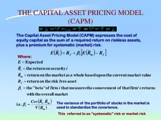
The Capital Asset Pricing Model. The Risk Return Relation Formalized. Summary. E(r) = r f + . = amount of risk premium per unit risk. Define the market portfolio as having one unit of risk, Var(r m ) = 1 unit of risk. Risk premium per unit of risk is then E(r m ) – r f .

E N D
The Capital Asset Pricing Model The Risk Return Relation Formalized
Summary • E(r) = rf + . • = amount of risk premium per unit risk. • Define the market portfolio as having one unit of risk, Var(rm) = 1 unit of risk. • Risk premium per unit of risk is then E(rm) – rf. • Any asset contributes to Var(rm) (in a w.d. port.) not by Var(ri) or STD (ri) but Cov(ri, rm). • Standardize Cov(ri, rm) by Var(rm) (to get it as the number of “units”) and get i as the measure of risk of any asset i. • Then: E(ri) = rf + i (E(rm) – rf) the famous SML.
Risk and Return • When there is only one asset its risk and return can be measured as we discussed using expected return and variance or standard deviation. • If there is more that one asset (and so we can form portfolios) risk and return are more complex. • We will show there are two types of risk for individual assets: • Diversifiable/nonsystematic risk/idiosyncratic • Nondiversifiable/systematic/market risk • We can eliminate diversifiable risk without cost by combining assets into portfolios. • It is usually possible to improve the risk/return tradeoff offered by any single asset by diversifying.
Summary: Risk and Return for Portfolios • (i) A portfolio’s expected return is always a weighted average of the expected returns of the portfolio's component assets. • (ii) The risk of a portfolio's return, as measured by the standard deviation of its returns, is almost always less than the weighted average of the total risks of its component assets. This is the powerful force of diversification. • (iii) Risk generally declines when new assets are added to a portfolio. Risk declines more the lower the correlations between the new asset's payoff (return) and the payoffs (returns) to the assets already in the portfolio. • (iv) For individual assets only the risk that contributes to the risk of a well diversified portfolio requires a premium.
Diversification Example: Writing Maritime Insurance • Suppose we are in the business of insuring oil tankers. Each tanker is insured for $10.3 million, and the owner pays us a $300,000 insurance premium per boat. The probability of a tanker sinking is 1.1%. • Our expected gain is positive but it is a highly risky position!
Now suppose we insure 1/2 of two separate boats instead of all of one boat. • What is happening here?
Diversification and Insurance • If we insure 1/30 of 30 boats • Expected payoff = 0.1867 • Standard Deviation = 0.196 • If we insure 1/100 of 100 boats • Expected payoff = 0.1867 • Standard Deviation = 0.107 • If we insure a tiny part of each of an infinite number of boats? • An important feature of the example is that outcomes, whether boats sink, were assumed to be uncorrelated across boats. • More generally, the degree of diversification benefit depends on the correlation among the payoffs on the different assets.
Diversification and Insurance • What would happen if we insure two boats but both boats sailed the same route, chained together? • In financial markets the returns on most assets are positively correlated and so we cannot get rid of all of the risk with diversification. However, we can get rid of quite a bit.
Covariances and Correlations: The Keys to Understanding Diversification • When thinking in terms of probability distributions, the covariance between the returns of two assets’ (A and B) Covariance = Cov(A,B) = AB = • When estimating covariances from historical data, the estimate is given by: • Note: An asset’s variance is its covariance with itself.
Correlation Coefficients • Covariances are difficult to interpret. Only the sign is really informative. Is a covariance of 20 big or small? The correlation coefficient, , is a normalized version of the covariance given by: • Correlation = CORR(A,B) = • The correlation will always lie between 1 and -1. • A correlation of 1.0 implies ... • A correlation of -1.0 implies ... • A correlation of 0.0 implies ...
Risk and Return in Portfolios: Example • Two Assets, A and B • A portfolio, P, comprised of 50% of your total investment • invested in asset A and 50% in B. • Only five equally probable future outcomes, summarized below. • In this case: • VAR(A) = 191.6, STD(A) = 13.84, and E(rA) = 16%. • VAR(B) = 106.0, STD(B) = 10.29, and E(rB) = 12%. • COV(A,B) = 21 • CORR(A,B) = 21/(13.84*10.29) = .1475. • VAR(P) = 84.9, STD(P) = 9.21, E(rp) = ½ E(rA) + ½ E(rB) = 14% • Var(P) or STD(P) is less than that of either component!
What risk return combinations would be possible with different weights? Asset A • ½ and ½ portfolio • Asset B •
What risk return combinations would be possible with a different correlation between A and B? Asset A • Asset B •
Symbols: Variance of a Two-Asset Portfolio For a portfolio of two assets, A and B, the portfolio variance is: Or, For the two-asset example considered above: Portfolio Variance = .52(191.6) + .52(106.0) + 2(.5)(.5)21 = 84.9 (check for yourself)
For General Portfolios • The expected return on a portfolio is the weighted average of the expected returns on each asset. If wi is the proportion of the investment invested in asset i, then • Note that this is a ‘linear’ relationship.
Risk in N-asset Portfolios • For N assets there are: • N variances (one per asset). • (N2 - N)/2 different covariances. One between each unique pair of assets. • technical note: COV(A,B) = COV(B,A) • The variance of the portfolio return is the weighted average of all these variances and covariances. • Each variance is weighted by the square of the portfolio weight for that asset (just like the two asset case). • Each covariance is weighted by twice the product of the weights for the two assets involved (again, just as before). • The risk (standard deviation) of the portfolio return will generally be less than the weighted average of the standard deviations of the components. • “Generally” means will beunless the assets are all perfectly correlated.
What happens when the number of assets in the portfolio, N, becomes large? • This is easiest to demonstrate if we assume: • that all the assets have the same variance of return, VAR. • The covariance between all pairs of assets is the same, COV. • The portfolio is equal-weighted (each asset has a weight 1/N) • Then, Portfolio Return Variance is: (1/N)VAR + (1 - 1/N)COV • What happens if n approaches infinity? • Is the average covariance between all assets a positive or negative number? • This tells us that it is an assets covariance with the return on a portfolio that determines its contribution to portfolio risk. • Graphical Illustration in the case where VAR = 100:
Portfolio standard deviation Nonsystematic risk Systematic/Market risk Number of 5 10 securities DIVERSIFICATION ELIMINATES UNIQUE RISK Diversification is costless!!
Diversification • Diversification reduces risk. If asset returns were uncorrelated on average, diversification could eliminate all risk. They are actually positively correlated on average. • Diversification will reduce risk but will not remove all of the risk. So, • There are two kinds of risk • Diversifiable/nonsystematic/idiosyncratic risk. • Disappears in well diversified portfolios. • It disappears without cost, i.e. you need not sacrifice expected return to reduce this type of risk. • Nondiversifiable/systematic/market risk. • Does not disappear in well diversified portfolios. • You have to sacrifice expected return to reduce your exposure to systematic risk.
Nonsystematic/diversifiable risks • Examples • Firm discovers a gold mine beneath its property • Lawsuits • Technological innovations • Labor strikes • The key is that these events are random and unrelated across firms. Some surprises are positive, some are negative. On average, across firms, the surprises offset each other if your portfolio is made up of a large number of assets.
Systematic/Nondiversifiable risk • We know that the returns on different assets are positively correlated with each other on average. This suggests that economy-wide influences affect all assets. • Examples: • Business Cycle • Inflation Shocks • Productivity Shocks • Interest Rate Changes • Major Technological Change • These are economic events that affect all assets. The risk associated with these events is systematic, and does not disappear in well diversified portfolios.
Measuring Systematic Risk • How can we estimate the amount or proportion of an asset's risk that is diversifiable or non-diversifiable? • The Beta Coefficient is the slope coefficient in an OLS regression of stock returns on market returns: • As such, Beta is a measure of sensitivity: it describes how strongly the stock return moves with the market. • Example: A Stock with = 2 will on average go up 20% when the market goes up 10%, and vice versa.
Some Additional Insight: Restate Beta in terms of correlations. • Since CORR(Ri,Rm) = COV(Ri,Rm)/STD(Rm)STD(Ri), the market beta can be restated as: • i = STD(Ri)CORR(Ri,Rm)/STD(Rm). • Interpret the components this way: • STD(Ri) is a measure to the total risk of asset i. • CORR(Ri,Rm) is a measure of the proportion of asset i's risk that is systematic. • STD(Ri)CORR(Ri,Rm) measures the systematic risk of asset i. • STD(Rm) measures the total risk of the market, all of which is systematic. • So, i is the systematic risk of asset i, relative to the systematic risk of the market. • This also implies that the average of all betas is 1.0, as is the market’s.
Betas and Portfolios • The Beta of a portfolio is the weighted average of the component assets’ Betas. • Example: You have 30% of your money in Asset X, which has X = 1.4 and 70% of your money in Asset Y, which has Y = 0.8. • Your portfolio Beta is: P = .30(1.4) + .70(0.8) = 0.98. • Why do we care about this feature of betas? • It shows directly that an asset’s beta measures the contribution that asset makes to the risk of a portfolio! • Also note that this is a linear (simple) relation.
Recap: What is Beta? (1) A measure of the sensitivity of a stock’s return to market returns. (2) A measure of a stock’s systematic risk (relative to the average or the market). (3) A standardized measure of the contribution of this stock to the risk of a well diversified portfolio.
How To Get Beta. • We estimate beta using a regression equation. • In practice, generally use last five years of monthly data. Some companies publish beta estimates on a regular basis: • Value Line, Merrill Lynch Beta Book, S&P • What if the company is not publicly traded? • Find a comparable company that is traded. • Use accounting data (ROE) instead of stock returns. • Reason it out.
Microsoft return % 30 25 20 Beta = 1.2 15 10 • 10 • 5 10 Mkt return % • 5 • 15 • 20 ESTIMATING MICROSOFT'S BETA
What Determines Beta? • Beta is a measure of sensitivity to the market. • Companies with cyclical cash flows will tend to have higher betas. • Higher operating leverage implies higher betas. • Operating leverage is the ratio of fixed costs to variable costs. • Higher financial leverage also means higher equity beta (more on this later).
Betas for selected common stocks Stock Beta Stock Beta AT&T .96 Ford 1.03 Boston Edison .49 Home Depot 1.34 Bristol-Myers Squibb .92 McDonald's 1.06 Delta Airlines 1.31 Microsoft 1.20 Digital Equipment 1.23 Nynex .77 Dow Chemical 1.05 Polaroid .96 Exxon .46 Tandem Comp. 1.73 Merck 1.11 UAL 1.84
The Capital Asset Pricing Model (CAPM) • Given that • some risk can be diversified, • diversification is easy and costless, • rational investors diversify, • there should be no premium associated with diversifiable risk. • What is the equilibrium relation between risk and expected return in the capital markets? • The CAPM is the best-known and most-widely used equilibrium model of the risk/return relation.
CAPM Intuition • E[Ri] = RF (risk free rate) + Risk Premium = Appropriate Discount Rate • Risk free assets earn the risk-free rate (think of this as a rental rate on capital). • If the asset is risky, we need to add a risk premium. • The size of the risk premium depends on the amount of systematic risk for the asset (stock, bond, or investment project) and the price per unit risk. • Could a risk premium ever be negative?
Number of units of systematic risk (b) Market Risk Premium or the price per unit risk The CAPM Intuition Formalized or, • The expression above is referred to as the “Security Market Line” (SML).
Applying the CAPM to select a discount rate • Three inputs are required: (i) An estimate of the risk free interest rate. • The current yield on short term treasury bills is one proxy. • Practitioners tend to favor the current yield on longer-term treasury bonds but this may be a fix for a problem we don’t fully understand. • Remember to adjust the market risk premium accordingly. (ii) An estimate of the market risk premium, E(Rm - rf). • Expectations are not observable. • Generally use a historically estimated value. (iii) An estimate of beta. Is the project or a surrogate for it traded in financial markets? If so, gather data and run an OLS regression. If not, you enter a very fuzzy area.
The Market Risk Premium • The market is defined as a portfolio of all wealth including real estate, human capital, etc. • In practice, a broad based stock index, such as the S&P 500 or the portfolio of all NYSE stocks, is generally used The Market Risk Premium Is Defined As: • Historically, the market risk premium has been about 9% above the return on treasury bills • The market risk premium has been about 7% above the return on treasury bonds • Is the expected risk premium smaller today?
Physical Assets Versus Securities • How does the SML help the firm to select assets. • The SML defines the rate of return required by the firm’s shareholders. The firm should select assets that will earn more than the rate of return required by the firm’s shareholders. • These assets are precisely those that have positive NPV when discounted at the rate given by the SML. • Where would a positive NPV asset plot relative to the SML?
SML: Ri = RF + bi( E[RM] - RF ) Expected Return (%) RM RF 1.0 Risk: bi The Security Market Line
BK INDS REVISITED • ValueLine on Tektronix: beta = 1.0585 (Tektronix and BK Inds). • BK Inds is a lot like Tektronix in terms of activities/operations/ asset structure. The beta risk of BK Inds overall, as it turns out, is the same. • Assume same amount of debt in capital structure (later). • Suppose RF = 3.5% and the recent risk premium has been 7%. • Then expected return on both Tektronix and BK Inds should be E(RBK) = .035 + 1.0585 X .07 = .1091.
BK INDS REVISITED • Thus, the appropriate discount rate on BK Inds is 10.91% if the new project looks like the conglomeration of old projects. NPV = $4,237,972 • Note: both Tektronix and BK Inds also have activities in marine power, pleasure boating, defense, fishing tackle, etc. Are text editing systems likely to be similar in terms of risk? Probably not!
BK INDS REVISITED • What to do? It turns out that there is another company that makes text editing systems in another region with similar economic and demographic characteristics. The beta of Symtec, Ltd. is 1.35. This might provide a reasonable comparison for risk. Then the discount rate should be • E(RBK) = .035 + 1.35 X .07 = .1295, or 12.95%. NPV = $2,310,4889
Summary • Find comparables with similar risk to the project being evaluated. • Similar risk means similar beta. • Calculate discount rate from the SML to get required rate of return for equityholders. • Use the discount rate to discount the expected cash flows from the project. If the NPV exceeds zero, and you are satisfied with the sensitivity analysis you performed, proceed with the project. • You will need to adjust beta if the project has a different debt ratio than the comparable (later).