Download
1 / 29
290 likes | 425 Vues
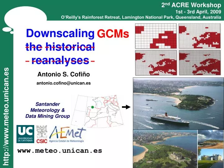
2 nd ACRE Workshop 1st - 3rd April, 2009 O’Reilly’s Rainforest Retreat, Lamington National Park, Queensland, Australia. GCMs. Downscaling the historical reanalyses. Antonio S. Cofiño antonio.cofino@unican.es. Santander Meteorology & Data Mining Group. www.meteo.unican.es.

E N D
2nd ACRE Workshop 1st - 3rd April, 2009 O’Reilly’s Rainforest Retreat, Lamington National Park, Queensland, Australia GCMs Downscaling the historical reanalyses Antonio S. Cofiño antonio.cofino@unican.es Santander Meteorology & Data Mining Group www.meteo.unican.es
Why Downscaling Methods? Interpolated Temp (20 km) Climatology (1961-90) ECHAM5/MPI-OM (200 km) AEMET TYPICAL SCALE OF GCMs REAL WORLD SCALE NEEDED FOR IMPACT STUDIES Global Predictions Emission Scenarios GCM
Downscaling Methodologies RCM Dynamical Downscaling runs regional climate models in reduced domains with boundary conditions given by the GCMs. B2 A2 Historical Records A2 Climatology (1961-90) Statistical Downscaling techniques are based on empirical models fitted to data using historical records. Y = f (X;) The form and parameters of the model depend of the different tecniques used. A2 Global Predictions Emission Scenarios GCM
Climate: Multi-Model, Multi-Scenario GCM Global Predictions Emission Scenarios
Dynamical Downscaling: RCMs Based on numerical models solving, at “high” temporal and spatial resolution, the primitive equations of the atmosphere. Usually the low resolution outputs from GCMs are used as Boundary Conditions and Initial Conditions for one-way nesting of a Local Area Model.
Dynamical Downscaling: RCMs • The results from RCMs are critically dependent on decisions about: • Spatial ant temporal resolution • The size and the position of the domain • The parameterizations of physical process • The Boundary Conditions • The Initial Conditions -> Internal variability Fernandez et al. (2007) J Geoph Res 112:D04101 “Sensitivity of MM5 to physical parameter ...” Jones et al. (1995) Q J R Meteorol Soc 121:1413 “Simulation of climate change over Europe ...” Vukicevic & Errico (1990) Mon Wea Rev 118:1460 “The influence of artificial and physical ...” Fernández (2004) PhD Diss. UPV/EHU “Statistical and dynamical downscaling models ...” GonzálezRouco et al. (2001) J Clim 14:964 “Quality Control and Homogeneity of Precip ...”Colle et al. (2000) Wea Forecasting 15:730 “MM5 precipitation verification over the Pacific ...”
ENSEMBLES. The SDS Portal Y = f (X;) http://www.meteo.unican.es/ensembles
Statistical Downscaling: Methods • Transfer-Function Approaches (generative) • Non-Generative Algorithmic Methods
Linear Regression Logistic Regression (T(1ooo mb),..., T(500 mb); Z(1ooo mb),..., Z(500 mb); .......; H(1ooo mb),..., H(500 mb)) = Xn Yn Linear Regression: Yn= aXn+ b Suitable for probabilistic forecast with a simple modification: P(precip>10mm) Logistic Regression Yn= F(aXn+ b) Predictands: precip., etc. for day n Gridded Atmospheric Patterns for day n
Selection of Predictors EOF 1 EOF 2 EOF 3 EOF 4
Linear & Logistic Regression Wind Speed [0,¥) P(Wind Speed >50km/h) [0,1] Observations from 1977- 2002. ERA40 over 27 grid points for the same period (60% for trainning and 40% for validation)
Artificial Neural Networks Artificial Neural Networks are inspired in the structure and functioning of the brain, which is a collection of interconnected neurons (the simplest computing elements performing information processing): • Each neuron consists of a cell body, that contains a cell nucleus. • There are number of fibers, called dendrites, and a single long fiber called axon branching out from the cell body. • The axon connects one neuron to others (through the dendrites). • The connecting junction is called synapse.
Functioning of a “Neuron” • The synapses releases chemical transmitter substances. • The chemical substances enter the dendrite, raising or lowering the electrical potential of the cell body. • When the potential reaches a threshold, an electric pulse or action potential is sent down to the axon affecting other neurons.(Therefore, there is a nonlinear activation). • Excitatory and inhibitory synapses. weights (+ or -, excitatory or inhibitory) neuron potential: mixed input of neighboring neurons (threshold) nonlinear activation function
1. Init the neural weight with random values2. Select the input and output data and train it3. Compute the error associate with the output 4. Compute the error associate with the hidden neurons 5. Compute and update the neural weight according to these values Multilayer Perceptron (Feed-forward) x h y hi InputsOutputs Gradient descent The neural activity (output) is given by a no linear function.
Model 1: Regression • Model 2: Neural Network Regression vs. Neural Networks Wind Speed [0,¥) Observations from 1977- 2002. ERA40 over 27 grid points for the same period 60% for trainning and 40% for validation
Analogs & Weather Typing Analog set PC2 PC1 Weather Type (cluster) The probabilistic local prediction is obtained from the relative frequency of snow occurrence (binary variable) in the analog set or cluster.
Comparison of Techniques: Wind Model 1 Model 2 Model 1 Model 2 P(12 ) P=(P(06),P(12),P(18),P(24),P(30)) P(Wind Speed >50km/h) [0,1] Observations from 1977- 2002. ERA40 over 27 grid points for the same period 60% for trainning and 40% for validation • Logistic Regression • Neural Network 10 PCs:5:1 • Analogs, k-NN (k=50)
Probabilistic Weather Typing Weather Type (cluster) x1 x2 x3 x4 x5 ... The application to an EPS requires applying the method to each of the ensemble members: Prob(x) Mean(x) Aggregation of results Pforecast (precip > u) = SCk P(precip > u | Ck) Pforecast(Ck)
Validation of Regional Projections Precipitation Perú 50 Km Downscaling needed ! Observations: Seasonal precip. during DJF 1997/98 at Morropón: 1300 mm, Sausal: 360 mm. Predictions (DEMETER): Analysis and Downscaling Multi-Model Seasonal Forecasts in Peru using Self-Organizing Maps by J. M. Gutiérrez, R. Cano, A. S. Cofiño, and C. Sordo, Tellus 57A, 435-447 (2005).
Skill of the Downscaling Method Numeric Forecast: Precip = * Probabilistic: P(precip>u)=* U = Percentile 80 U= Percentile 90
Conclusions • End-User applications require downscaled data: spatial, temporal and parameters • 2 approaches: • Dynamical: parameterization tuning, high costs in terms of computer resources, can provide downscaled data where no observations are available,….. • Statistical: based on “past” observations, difficult to give a physical meaning, predictor selection issues, calibration of GCM, can provide non-linear relationships between predictors and predictands,… • Used for Climate change scenarios, Seasonal forecasting, Weather forecasting…and of course re-analysis applications
Questions? antonio.cofino@unican.es http://www.meteo.unican.es