Download
1 / 60
600 likes | 813 Vues
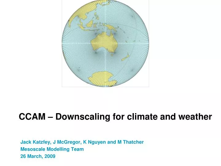
CCAM – Downscaling for climate and weather. Jack Katzfey, J McGregor, K Nguyen and M Thatcher Mesoscale Modelling Team 26 March, 2009. Outline. Dynamical Downscaling Techniques Impact of bias correction of SST and atmospheric forcing Climate Futures for Tasmania A2 and B1 scenarios

E N D
CCAM – Downscaling for climate and weather Jack Katzfey, J McGregor, K Nguyen and M Thatcher Mesoscale Modelling Team 26 March, 2009
Outline • Dynamical Downscaling Techniques • Impact of bias correction of SST and atmospheric forcing • Climate Futures for Tasmania • A2 and B1 scenarios • 6 GCMs • 140 years at 60 km • 140 years at 14 km • Specialised Weather Forecasts Dynamical Downscaling Techniques
Outline – Dynamical Downscaling Techniques • Motivation • Conformal Cubic Atmospheric Model (CCAM) • Climate Futures for Tasmania project (at least the downscaling bit) • Downscaling Techniques/Strategies • Preliminary Results • Conclusions • Acknowledgments to Climate Futures for Tasmania, Tasmanian Sustainable Yields, Climate Adaptation Flagship. Dynamical Downscaling Techniques
Motivation • There is a range of techniques to dynamically downscale • Models • Time-slice with high-resolution AGCMs • Stretched-grid models • Limited-area models • Inputs • Atmospheric forcing using various techniques • Ocean temperatures and Sea Ice • Atmospheric chemistry (aerosols, ozone, CO2) • This preliminary study attempts to analyse the impact of some of these techniques on the simulation of current climate and climate change Dynamical Downscaling Techniques
Downscaling Strategies GCM • Select GCM (scenario, data, performance) • Select model and grid (grid, resolution, stretching) • Bias-correct GCM SSTs? • Apply atmospheric forcing? Bias Corrected SST (BCTS) No Bias Corrected SST (TS) Forcing (BCTS, F) No Forcing (BCTS, NF) Forcing (TS, F) No Forcing (TS, NF)
Weighting/selection of GCM results Does it matter? How to do this? Based upon work of Ian Smith
Summary of model assessments: A: Number of rainfall criteria failed (Smith et al., 2008) B: Satisfied ENSO criteria (Min et al., 2005; van Oldenborough et al., 2005) C: Satisfied criteria for rainfall, temperature and MSLP (Suppiah et al., 2007) D: M-statistic representing goodness of fit at simulating rainfall, temperature and MSLP over Australia (Watterson, 2008) E: Satisfied criteria for daily rainfall over Australia (Perkins and Pitman, 2008) F: Satisfied criteria for daily rainfall over MDB region (Maximo et al., et al., 2008) G: Satisfied criteria for MSLP over MDB region (Charles et al., 2007) H: Below median errors for 14 variables (Reichler and Kim, 2008).
Downscaling Strategies Preliminary results shown today are from runs completed for: Only using CSIRO Mk3.5 GCM 10 Januaries and 10 Julys Current (1970-79) and Future (A2, 2080-89) Dynamical Downscaling Techniques • Questions: • Do we want/need to get current climate right to believe climate change projection? • Do we expect the Downscaled Climate Projection to be similar to GCM? Or can the Downscaled results improve upon the GCM? • What about inconsistency of corrected SSTs and uncorrected atmospheric field adjustment?
SSTbias correction MIROC Mk3.5 • The following plots show examples of January SST biases in different GCMs • One practice in regional climate modelling is to correct these biases before feeding the SSTs into regional models • Note that no changes are made to the variability in SSTs, nor to the rate of warming • Some regional modelling groups also re-run their atmospheric GCM once the SST bias is removed GFDL2.0 GFDL2.1 ECHAM5 HadCM3 Dynamical Downscaling Techniques
Conformal Cubic Atmospheric Model • CCAM was chosen as it does not require lateral boundary conditions due to its variable resolution conformal cubic grid • CCAM also supports various nudging techniques including • Spectral nudging • Davies style BCs • Global relaxation methods • SST only forcing • For this study a C64 grid was used (64x64x6 horizontal grid points) with 18 vertical levels Plot of grid resolution for the 60 km resolution regional climate study Dynamical Downscaling Techniques
Comparison of July rainfallNote: rainfall over tropics, improvement with bcSST, similarity of CCAM when using GCM SST Obs CSIRO Mk3.5 GCM CCAM bcSST, No Atmos. F. CCAM No bcSST, No Atmos. F. Dynamical Downscaling Techniques
Statistics Table 1. Statistics computed for rainfall versus observed climatology 10 Julys for Australian region (110 to 160 E longitudes, -10 to -45 S latitudes).
Change in July rainfall BCTS, NF BCTS, F • The following plots show changes in simulated July rainfall between the 1970-79 climate and 2080-89 climate (mm/d) • Experiment options are: • BCTS = Bias corrected SSTs • TS = SSTs without bias corrected • F = Spectral adjustment • NF = No atmospheric nudging • cont = continuous run • TS,F is closest to the host GCM TS, F TS, NF Mk3.5 BCTS, NF, cont Dynamical Downscaling Techniques
Conclusions • Preliminary investigation of the impact of different dynamical downscaling methodologies for simulating the Australian regional climate • Much more work exploring parameter space • Regional atmospheric simulations with bias corrected SSTs and no nudging are best able to model the 20th century climate • Nudging of atmospheric fields without bias correction to SSTs produces a regional climate whose large scale behaviour more closely resembles the host GCM • The ‘best’ method depends on the objectives of the regional simulation • How should we do dynamical downscaling? • Future work is directed towards understanding the implications of different downscaling techniques for estimating uncertainties in regional climate projections Dynamical Downscaling Techniques
Downscaling Strategies • Questions: • Do we want/need to get current climate right to believe climate change projection? • Do we expect the Downscaled Climate Projection to be similar to GCM? Or can the Downscaled results improve upon the GCM? • What about inconsistency of corrected SSTs and uncorrected atmospheric field adjustment? Dynamical Downscaling Techniques
Climate Futures for Tasmania A2 B1 ECHAM5 GFDL20 GFDL21 MIROC(medres) UKHADCM3 CSIRO Mk3.5 CCAM C64 60km BCTS, SI 140 year (1961-2100) • Modern regional climate projections are based on atmospheric and SST forcings from a variety of CMIP3 GCMs and for different SRES emission scenarios • The results are used to support a range of impact studies from which adaptation and mitigation studies can be developed CCAM C48 14km Digital filter 140 year (1961-2100)
14 km resolution simulations for Tasmania • 14 km resolution regional climate simulations for Tasmania are being generated using a multiple nesting technique • The host model used is the 60 km resolution CCAM simulation with bias corrected SSTs and no atmospheric nudging • The 14 km simulation employs the same bias corrected SSTs, but with spectral nudging to help correct errors arising outside the regional focus where the grid resolution is more coarse Stretched conformal cubic grid used for 14 km resolution simulations over Tasmania Dynamical Downscaling Techniques
Modelling the Local Scale (Tasmania) • One of the main reasons to downscale is the better representations of topography and its influence on the climate Global grid 2 cells 60 km grid 35 cells 14 km grid 860 cells
Tasmania wide mean annual daily maximum temperature (screen) Model mean of A2 and B1 runs, showing standard deviations
CSIRO Mk3.5 GFDL 2.0 GFDL 2.1 Mean daily Tmax (deg C) 2070:2099 – 1961:1990 A2 HadCM 3 ECHAM 5 MIROC medres Model Mean B1 Model Mean
Statewide mean annual total rainfall (1961-2100) 11 year running average A2 B1
Δ annual rainfall (mm), 2070-2099 minus 1961-1990 Model mean A2 Model mean B1
Change in SST (deg C): 2070:2099 minus 1961:1990 Model mean A2 B1
Conclusions • We now have a large range of 60 km Australia wide dynamical downscaled results • A2 and B1 scenarios • 6 different GCMS – 12 runs • CCAM run with bias corrected Sea Surface Temperatures and Sea Ice • Also have 12 runs at 14 km of downscaled results for Tasmania Dynamical Downscaling Techniques
Specialised Weather Forecasts • Rapid Deployment • Fast execution • ~2hr for 1day,1km fcst on laptop • High-resolution capable • Tailored output • Validation • 60km fcst has similar S1 score to GASP • Able to force TAPM • Pollution/dispersion • Applications • Predictwind(Rec. boat fcst.) • Alinghi (2 America’s Cup wins) • IRR (rapid response) • TasHydro(Cloud Seeding) • Olympic Sailing (Qingdao) 1 km zoomed into race area Windows Interface
www.cawcr.gov.au Ensemble One-kilometer Resolution Numerical Weather Forecasts for the America’s Cup Also: John McGregor and Marcus Thatcher Jack Katzfey Mesoscale Modelling Applications Team Leader 28 November 2008
Outline • Forecast requirements • Observations • Modelling • Example • Validation • Discussion The Centre for Australian Weather and Climate ResearchA partnership between CSIRO and the Bureau of Meteorology
Forecast Requirements • Morning Briefing (11am) • Synoptic situation • Ensemble predictions for race course (wd/ws) • Hour by hour forecast ws/wd – expected wind speed and trends • Other factors • Clouds/rain • Waves • Temperatures • Visible signs of expected changes? • Updated forecasts • Ensure all systems working • Compare forecast with observations, update forecast? The Centre for Australian Weather and Climate ResearchA partnership between CSIRO and the Bureau of Meteorology
Forecast Requirements • Last call (6 minutes before race start) • Expected wind speed/direction trends/changes for race (2.5 hours) • Expected wind speed/direction trends for 1st leg (5km, 45 minutes) • Variations of wind on race course • Wind left/right on course • Wind direction variations across course (esp. top – bottom) • Fans/bends • Mean wind speed and direction • Used by race boat to determine phase of shift (dir) and sail selection (spd) • Favoured end of start line • Confidence of forecast • Gain/loss associated with wind variations • How important to ‘get’ side • Comments • Small-scale shits unpredictable • Not measured well (even with dense buoy network) • Uncertain duration of shifts The Centre for Australian Weather and Climate ResearchA partnership between CSIRO and the Bureau of Meteorology
Outline • Forecast requirements • Observations The Centre for Australian Weather and Climate ResearchA partnership between CSIRO and the Bureau of Meteorology
Observations • Buoys (3 m masts) • Fixed location • Wind spd/dir every 15 sec (30 sec avg) • Pressure, temperature, relative humidity every 1 minute at 2 buoys • Weather boats (3 m masts, expect Wx1) • Movable, but also rocking – noisy • Wind spd/dir every 15 sec (30 sec avg) • MDS, RC, Alinghi • Wx1 has 24 m mast with wind sensors at 6,12,18, 24 m • Land • MDS (6) • Alinghi (8) • Profiler • Satellite • Radar But not many clouds/precipitation The Centre for Australian Weather and Climate ResearchA partnership between CSIRO and the Bureau of Meteorology
Surface Observations P,T WxB P,T WxB P,T P,T The Centre for Australian Weather and Climate ResearchA partnership between CSIRO and the Bureau of Meteorology Surface wind observations Circle is 10 km radius Diamond is race course
Outline • Forecast requirements • Observations • Modelling The Centre for Australian Weather and Climate ResearchA partnership between CSIRO and the Bureau of Meteorology
Model runs • CCAM runs in yellow The Centre for Australian Weather and Climate ResearchA partnership between CSIRO and the Bureau of Meteorology
Topography at 60km, 8km and 1km The Centre for Australian Weather and Climate ResearchA partnership between CSIRO and the Bureau of Meteorology
Outline • Forecast requirements • Observations • Modelling • Example The Centre for Australian Weather and Climate ResearchA partnership between CSIRO and the Bureau of Meteorology
Synoptic picture (PMSL and Sfc winds) The Centre for Australian Weather and Climate ResearchA partnership between CSIRO and the Bureau of Meteorology
High Resolution model predictions Forecast: 18 knots from 135° (watch for left trend late in day) The Centre for Australian Weather and Climate ResearchA partnership between CSIRO and the Bureau of Meteorology
Observations on race course Forecast: 18 knots from 135° (watch for left trend late in day) The Centre for Australian Weather and Climate ResearchA partnership between CSIRO and the Bureau of Meteorology
Outline • Forecast requirements • Observations • Modelling • Example • Validation • Distributions • Bias, Mean Abs. Error • Neighborhood verification techniques • Last call statistics The Centre for Australian Weather and Climate ResearchA partnership between CSIRO and the Bureau of Meteorology