Download
1 / 31
310 likes | 433 Vues
Long-Term Ambient Noise Statistics in the Gulf of Mexico. Mark A. Snyder & Peter A. Orlin Naval Oceanographic Office Stennis Space Center, MS Anthony I. Eller Science Applications International Corporation. EARS* Data. EARS Data Logger. Floats.

E N D
Long-Term Ambient NoiseStatisticsin theGulf of Mexico Mark A. Snyder & Peter A. Orlin Naval Oceanographic Office Stennis Space Center, MS Anthony I. Eller Science Applications International Corporation
EARS* Data EARS Data Logger Floats Bottom-moored omni-directional hydrophone Bandwidth of 10 Hz - 1000 Hz 14 months of data (Apr 2004 - May 2005) Water depth ~ 3200 meters Hydrophone depth ~ 2935 meters Vicinity 27.5 N, 86.1 W (about 159 nm south of Panama City, FL and 196 nm west of Tampa, FL) Acoustic Release * Environmental Acoustic Recording System
Location of EARS and NDBC* Weather Buoys 103 nm EARS 89 nm NDBC 42003 NDBC 42036 55 m 3200 m *National Data Buoy Center 3200 m
Monthly Trends
Monthly Statistics* • Mean • Median • Standard deviation • Skewness • Kurtosis • Coherence time** * For 8 third-octave bands. **Time for autocorrelation to decay to e-1 of its zero-lag value.
1 year cycle Hurricanes
Low frequency band Positive skewness Chi – Square PDF Apr04 May05
High frequency band Negative skewness Winter Storms Hurricanes Apr04 May05
1st order Gauss-Markov process is characterized by an exponentially-decaying autocorrelation. Coherence time = 2.97 hours
Power spectrum of 14-month time series shows how the energy associated with variability is spread over long and short time scales. • Each vertical bar = variance in each 1/10-decade* freq band. • Sum of all vertical bars = total variance. • Low frequency band • Most of the variability is in time scales near 10 hours • Red curve is plot of 1st order Gauss-Markov process * 1/10-decade≈ 1/3-octave 4 days 6 weeks 1 year
High frequency band • Most of the variability is in time scales near 100 hours 4 days 6 weeks 1 year
2 octaves to left and right of center frequency have correlation coefficient ≥ 0.5
A3 A1 A6 2.29 km 2.56 km Water depth = 3200 m at all 3 sites Hydrophone depth = 2935 m at all 3 sites 10 month comparison
100 Hz - more affected by local noise sources • 1000 Hz – wind is correlated over large distances • 100 Hz - more affected by local noise sources • 1000 Hz – wind is correlated over large distances
14-month avg wind speed = 11.3 knots • Avg significant wave height = 1.06 m • Avg Beaufort Wind Force = 3.5 • Moderate to heavy shipping • Shipping level 6-7 on scale of 1-9 • 14-month avg wind speed = 11.3 knots • Avg significant wave height = 1.06 m • Avg Beaufort Wind Force = 3.5 • Moderate to heavy shipping • (Shipping level = 6-7 on scale of 1-9, • with 1 = light, 9 = very heavy)
Best-Fit Density Functions (14 Months) σR = Rayleigh parameter. n = degrees of freedom.
14-Month Summary • Ambient noise at low frequencies (25 – 400 Hz) Mean > median > mode (2 – 3 dB spread) All 3 values close and predicted by moderate to heavy shipping. Location of all 3 caused positive skewness (skewed towards peaks). • Ambient noise at high frequencies (630 – 950 Hz) Mode > median > mean (2 – 3 dB spread) All 3 values close and predicted by avg BWF = 3.5 (11.3 knots avg wind). Location of all 3 caused negative skewness (skewed towards troughs).
14-Month Summary • Coherence time was low (2 – 4 hours) in shipping bands (25 – 400 Hz) • Coherence time was high (14 – 21 hours) in weather bands (630 – 950 Hz) • Monthly coherence time was highest during extreme wind conditions
14-Month Summary • Temporal variability occurred over 3 time scales: • 7 - 22 hours (shipping-related) • 56 - 282 hours (2 - 12 days, weather-related) • 8 - 12 months (1 year cycle) • The 25 Hz time series had a strong 8-hour component (sinusoidal autocorrelation; not shipping or weather) • The 50, 100 and 200 Hz frequency bands were fit by a 1st order Gauss-Markov process (well characterized by 3 parameters: mean, variance and coherence time) • More complicated structure in other bands
Avg BWF = 2.5 Mean = 56.26 dB σ = 5.78 dB Range = 38.27 dB Skewness = 0.45 C.T. = 1.74 hours Avg BWF = 4 Mean = 62.73 dB σ = 4.67 dB Range = 31.81 dB Skewness = -0.51 C.T. = 10.31 hours
Data Processing Raw Acoustic Time Series Data 2048 Point FFT 10 Minute Avg Power Spectra Separate Data Into 14 Months Sampled at 2.5 kHz. Remove disk spin and clips. Δf = 1.22 Hz. Average 732 (0.82 seconds each) periodograms. Bandpass Each Month’s Data Over Eight 1/3-Octave Bands Compute Monthly Statistics Over Each Frequency Band FC = 25, 50, 100, 200, 400, 630, 800, 950 Hz Compute the average power in each band every 10 minutes.
Frances Ivan I Ivan II Jeanne