Download
1 / 33
330 likes | 575 Vues
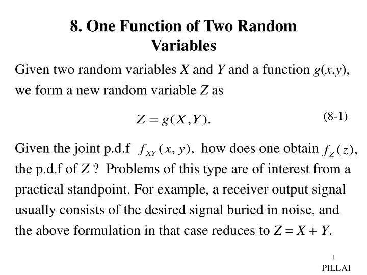
8. One Function of Two Random Variables . Given two random variables X and Y and a function g ( x , y ), we form a new random variable Z as

E N D
8. One Function of Two Random Variables Given two random variables X and Y and a function g(x,y), we form a new random variable Z as Given the joint p.d.f how does one obtain the p.d.f of Z ? Problems of this type are of interest from a practical standpoint. For example, a receiver output signal usually consists of the desired signal buried in noise, and the above formulation in that case reduces to Z = X + Y. (8-1) PILLAI
It is important to know the statistics of the incoming signal for proper receiver design. In this context, we shall analyze problems of the following type: Referring back to (8-1), to start with (8-2) (8-3) PILLAI
where in the XY plane represents the region such that is satisfied. Note that need not be simply connected (Fig. 8.1). From (8-3), to determine it is enough to find the region for every z, and then evaluate the integral there. We shall illustrate this method through various examples. Fig. 8.1 PILLAI
Example 8.1: Z = X + Y. Find Solution: since the region of the xy plane where is the shaded area in Fig. 8.2to the left of the line Integrating over the horizontal strip along the x-axis first (inner integral) followed by sliding that strip along the y-axis from to (outer integral) we cover the entire shaded area. (8-4) Fig. 8.2 PILLAI
We can find by differentiating directly. In this context, it is useful to recall the differentiation rule in (7-15) - (7-16) due to Leibnitz. Suppose Then Using (8-6) in (8-4) we get Alternatively, the integration in (8-4) can be carried out first along the y-axis followed by the x-axis as in Fig. 8.3. (8-5) (8-6) (8-7) PILLAI
In that case and differentiation of (8-8) gives (8-8) (8-9) Fig. 8.3 If X and Y are independent, then and inserting (8-10) into (8-8) and (8-9), we get (8-10) (8-11) PILLAI
The above integral is the standard convolution of the functions and expressed two different ways. We thus reach the following conclusion: If two r.vs are independent, then the density of their sum equals the convolution of their density functions. As a special case, suppose that for and for then we can make use of Fig. 8.4 to determine the new limits for Fig. 8.4 PILLAI
In that case or On the other hand, by considering vertical strips first in Fig. 8.4, we get or if X and Y are independent random variables. (8-12) (8-13) PILLAI
Example 8.2: Suppose X and Y are independent exponential r.vs with common parameter , and let Z = X + Y. Determine Solution: We have and we can make use of (13) to obtain the p.d.f of Z = X + Y. As the next example shows, care should be taken in using the convolution formula for r.vs with finite range. Example 8.3: X and Y are independent uniform r.vs in the common interval (0,1). Determine where Z = X + Y. Solution: Clearly, here, and as Fig. 8.5 shows there are two cases of z for which the shaded areas are quite different in shape and they should be considered separately. (8-14) (8-15) PILLAI
Fig. 8.5 For For notice that it is easy to deal with the unshaded region. In that case (8-16) (8-17) PILLAI
Using (8-16) - (8-17), we obtain By direct convolution of and we obtain the same result as above. In fact, for (Fig. 8.6(a)) and for (Fig. 8.6(b)) Fig 8.6 (c) shows which agrees with the convolution of two rectangular waveforms as well. (8-18) (8-19) (8-20) PILLAI
Fig. 8.6 (c) PILLAI
Fig. 8.7 Example 8.3: Let Determine its p.d.f Solution: From (8-3) and Fig. 8.7 and hence If X and Y are independent, then the above formula reduces to which represents the convolution of with (8-21) (8-22) PILLAI
As a special case, suppose In this case, Z can be negative as well as positive, and that gives rise to two situations that should be analyzed separately, since the region of integration for and are quite different. For from Fig. 8.8 (a) and for from Fig 8.8 (b) After differentiation, this gives (a) (8-23) Fig. 8.8 (b) PILLAI
(a) (b) Example 8.4: Given Z = X / Y, obtain its density function.Solution: We have The inequality can be rewritten as if and if Hence the event in (8-24) need to be conditioned by the event and its compliment Since by the partition theorem, we have and hence by the mutually exclusive property of the later two events Fig. 8.9(a) shows the area corresponding to the first term, and Fig. 8.9(b) shows that corresponding to the second term in (8-25). (8-24) (8-25) Fig. 8.9 PILLAI
Integrating over these two regions, we get Differentiation with respect to z gives Note that if X and Y are nonnegative random variables, then the area of integration reduces to that shown in Fig. 8.10. (8-26) (8-27) Fig. 8.10 PILLAI
This gives or Example 8.5: X and Y are jointly normal random variables with zero mean so that Show that the ratio Z = X / Y has a Cauchy density function centered at Solution: Inserting (8-29) into (8-27) and using the fact that we obtain (8-28) (8-29) PILLAI
where Thus which represents a Cauchy r.v centered at Integrating (8-30) from to z, we obtain the corresponding distribution function to be Example 8.6: Obtain Solution: We have (8-30) (8-31) (8-32) PILLAI
But, represents the area of a circle with radius and hence from Fig. 8.11, This gives after repeated differentiation As an illustration, consider the next example. (8-33) (8-34) Fig. 8.11 PILLAI
Example 8.7 : X and Y are independent normal r.vs with zero Mean and common variance Determine for Solution: Direct substitution of (8-29) with Into (8-34) gives where we have used the substitution From (8-35) we have the following result: If X and Y are independent zero mean Gaussian r.vs with common variance then is an exponential r.vs with parameter Example 8.8 : Let Find Solution: From Fig. 8.11, the present case corresponds to a circle with radius Thus (8-35) PILLAI
And by repeated differentiation, we obtain Now suppose X and Y are independent Gaussian as in Example 8.7. In that case, (8-36) simplifies to which represents a Rayleigh distribution. Thus, if where X and Y are real, independent normal r.vs with zero mean and equal variance, then the r.v has a Rayleigh density. W is said to be a complex Gaussian r.v with zero mean, whose real and imaginary parts are independent r.vs. From (8-37), we have seen that its magnitude has Rayleigh distribution. (8-36) (8-37) PILLAI
What about its phase Clearly, the principal value of lies in the interval If we let then from example 8.5, U has a Cauchy distribution with (see (8-30) with ) As a result To summarize, the magnitude and phase of a zero mean complex Gaussian r.v has Rayleigh and uniform distributions respectively. Interestingly, as we will show later, these two derived r.vs are also independent of each other! (8-38) (8-39) (8-40) PILLAI
Let us reconsider example 8.8 where X and Y have nonzero means and respectively. Then is said to be a Rician r.v. Such a scene arises in fading multipath situation where there is a dominant constant component (mean) in addition to a zero mean Gaussian r.v. The constant component may be the line of sight signal and the zero mean Gaussian r.v part could be due to random multipath components adding up incoherently (see diagram below). The envelope of such a signal is said to have a Rician p.d.f. Example 8.9: Redo example 8.8, where X and Y have nonzero means and respectively. Solution: Since substituting this into (8-36) and letting Multipath/Gaussian noise Line of sight signal (constant) Rician Output PILLAI
we get the Rician probability density function to be where is the modified Bessel function of the first kind and zeroth order. Example 8.10: Determine Solution: The functions max and min are nonlinear (8-41) (8-42) PILLAI
operators and represent special cases of the more general order statistics. In general, given any n-tuple we can arrange them in an increasing order of magnitude such that where and is the second smallest value among and finally If represent r.vs, the function that takes on the value in each possible sequence is known as the k-th order statistic. represent the set of order statistics among n random variables. In this context represents the range, and when n = 2, we have the max and min statistics. (8-43) (8-44) PILLAI
Returning back to that problem, since we have (see also (8-25)) since and are mutually exclusive sets that form a partition. Figs 8.12 (a)-(b) show the regions satisfying the corresponding inequalities in each term above. (8-45) Fig. 8.12 PILLAI
Fig. 8.12 (c) represents the total region, and from there If X and Y are independent, then and hence Similarly Thus (8-46) (8-47) (8-48) PILLAI
Once again, the shaded areas in Fig. 8.13 (a)-(b) show the regions satisfying the above inequalities and Fig 8.13 (c) shows the overall region. (c) (a) (b) Fig. 8.13 From Fig. 8.13 (c), where we have made use of (7-5) and (7-12) with and (8-49) PILLAI
Example 8.11: Let X and Y be independent exponential r.vs with common parameter . Define Find Solution: From (8-49) and hence But and so that Thus min ( X, Y ) is also exponential with parameter 2. Example 8.12: Suppose X and Y are as give in the above example. Define Determine (8-50) PILLAI
Solution: Although represents a complicated function, by partitioning the whole space as before, it is possible to simplify this function. In fact As before, this gives Since X and Y are both positive random variables in this case, we have The shaded regions in Figs 8.14 (a)-(b) represent the two terms in the above sum. (8-51) (8-52) (a) (b) Fig. 8.14 PILLAI
From Fig. 8.14 Hence Example 8.13 (Discrete Case): Let X and Y be independent Poisson random variables with parameters and respectively. Let Determine the p.m.f of Z. (8-53) (8-54) Fig. 8.15 PILLAI
Solution: Since X and Y both take integer values the same is true for Z. For any gives only a finite number of options for X and Y. In fact, if X = 0, then Y must be n; if X = 1, then Y must be n-1, etc. Thus the event is the union of (n + 1) mutually exclusive events given by As a result If X and Y are also independent, then and hence (8-55) (8-56) PILLAI
(8-57) Thus Z represents a Poisson random variable with parameter indicating that sum of independent Poisson random variables is also a Poisson random variable whose parameter is the sum of the parameters of the original random variables. As the last example illustrates, the above procedure for determining the p.m.f of functions of discrete random variables is somewhat tedious. As we shall see in Lecture 10, the joint characteristic function can be used in this context to solve problems of this type in an easier fashion. PILLAI