Download

1 / 61
820 likes | 1.41k Vues
HWRF Ocean: The Princeton Ocean Model (POM-TC). Richard M. Yablonsky University of Rhode Island WRF for Hurricanes Tutorial NCWCP, College Park, MD 14-16 January 2014. What is the Princeton Ocean Model?.

E N D
HWRF Ocean: The Princeton Ocean Model (POM-TC) Richard M. Yablonsky University of Rhode Island WRF for Hurricanes Tutorial NCWCP, College Park, MD 14-16 January 2014
What is the Princeton Ocean Model? • Three-dimensional, primitive equation, numerical ocean model (commonly known as POM; Mellor 2004) • Originally developed by Alan Blumberg and George Mellor in the late 1970’s • Initially used for coastal ocean circulation applications Open to the community during the 1990’s and 2000’s • Many user-generated changes incorporated into “official” code version housed at Princeton University
Developing HWRF Ocean (POM-TC) • Available POM code version transferred to University of Rhode Island (URI) in mid-1990’s • POM code changes made at URI specifically to address ocean response to hurricane wind forcing • This POM version coupled to GFDL hurricane model at URI • Coupled GFDL/POM model operational at NCEP in 2001 • Additional POM upgrades made at URI during 2000’s (e.g. initialization) and implemented in operational GFDL/POM • Same version of POM coupled to operational HWRF in 2007 • This POM version is now designated “POM-TC” • Some further POM-TC upgrades made at URI since 2007
Why Couple POM-TC to HWRF? • To create accurate SST field for input into the HWRF • Evaporation (moisture flux) from sea surface provides heat energy to drive a hurricane • Available energy decreases if storm-core SST decreases • Uncoupled hurricane models with static SST neglect SST cooling during integration high intensity bias • One-dimensional (vertical-only) ocean models neglect upwelling and horizontal advection, both of which can impact SST during integration (e.g. Yablonsky and Ginis 2009, 2013, Monthly Weather Review)
Physics of Storm-Core SST Change • Vertical mixing/entrainment (Slide 7) • Upwelling (Slide 8) • Horizontal advection (Slide 9) • Heat flux to the atmosphere (small by comparison)
A T M O S P H E R E 1) Vertical mixing/entrainment Wind stress → surface layer currents Current shear → turbulence Turbulent mixing → entrainment of cooler water POM-TC uses the Mellor-Yamada 2.5 turbulence closure submodel to parameterize vertical mixing O C E A N Warm sea surface temperature Sea surface temperature decreases Cool subsurface temperature Subsurface temperature increases This is a 1-D (vertical) process
A T M O S P H E R E 2) Upwelling Cyclonic wind stress → divergent surface currents Cyclonic hurricane vortex Divergent currents → upwelling Upwelling → cooler water brought to surface O C E A N Warm sea surface temperature Cool subsurface temperature This is a 3-D process
A T M O S P H E R E 3) Horizontal advection Preexisting cold pool is located outside storm core Cyclonic hurricane vortex Preexisting current direction is towards storm core Ocean currents advect cold pool under storm core O C E A N Warm sea surface temperature Cool subsurface temperature This is a horizontal process
A T M O S P H E R E Prescribed propagation speed Cyclonic hurricane vortex < < < < < < < < O C E A N Homogeneous initial SST < < < < Horizontally-homogeneous subsurface temperature What is the impact of varying storm translation speed?
2.4 m s-1 4.8 m s-1 Hurricanes have historically propagated in the Gulf of Mexico: < 5 m s-1 73% and < 2 m s-1 16% of the time And in the western tropical North Atlantic: < 5 m s-1 62% and < 2 m s-1 12% of the time So 3-D effects (e.g. upwelling) are important Yablonsky and Ginis (2009, Mon. Wea. Rev.)
3-D 1-D 2.4 m s-1 3-D 1-D 4.8 m s-1
Impact of Horizontal Advection: Example with a Warm Ocean Eddy SST & current vectors: 96-hour forecast 60-km SST cooling 200-km SST cooling Central Pressure Storm Track Yablonsky and Ginis (2013, Mon. Wea. Rev.)
POM-TC Atlantic Domains:“United” and “East Atlantic” 47.5°N ~18-km grid spacing 225 254 10.0°N 98.5°W 50°W 157 60°W 30°W
POM-TC 1D E-W Relocatable“East Pacific” Domain 40.0°N ~18-km grid spacing 241 241 0.0°N
POM-TC Sigma Vertical Coordinate • 23 vertical sigma levels; free surface (η) • Level placement scaled based on ocean bathymetry • Largest vertical spacing occurs where ocean depth is 5500 m • Location of 23 half-sigma levels when ocean depth is 5500 m: • 5, 15, 25, 35, 45, 55, 65, 77.5, 92.5, 110, 135, 175, 250, 375, • 550, 775, 1100, 1550, 2100, 2800, 3700, 4850, and 5500 m
Arakawa-C Grid: External Mode Plan View • Horizontal spatial differencing occurs on staggered Arakawa-C grid • 2-D variables “UA” and “VA” are calculated at shifted location from “η”
Arakawa-C Grid: Internal Mode Plan View • Horizontal spatial differencing occurs on staggered Arakawa-C grid • 3-D variables “U” and “V” are calculated at shifted location from “T” and “Q” • “T” here represents variables “T”, “S”, and “RHO” • “Q” here represents variables “Km”, “Kh”, “Q2”, and “Q2l”
Vertical Grid: Internal Mode Elevation View • Vertical spatial differencing also occurs on staggered grid • 3-D variables “W” and “Q” are calculated at shifted depth from “T” and “U” • “T” here represents variables “T”, “S”, and “RHO” • “Q” here represents variables “Km”, “Kh”, “Q2”, and “Q2l”
Time Stepping • POM-TC has a split time step • External (two-dimensional) mode uses short time step: • 22.5 seconds during pre-coupled POM-TC initialization • 13.5 seconds during coupled POM-TC integration • Internal (three-dimensional) mode uses long time step: • 15 minutes during pre-coupled POM-TC initialization • 9 minutes during coupled POM-TC integration • Horizontal time differencing is explicit • Vertical time differencing is implicit
POM-TC initialization • Prior to coupled model integration of HWRF/POM-TC, POM-TC must be initialized with a realistic, 3-D temperature (T) and salinity (S) field • This T & S field must then be used to generate realistic ocean currents via geostrophic adjustment • The “spun-up” ocean must then incorporate the preexisting hurricane-generated cold wake by applying TC’s wind stress using the NHC hurricane message file
Why is the cold wake “not as cold” here? Answer: We must look under the ocean surface!
Typical of Gulf of Mexico in Summer & Fall Typical of Caribbean in Summer & Fall
Approximate Locations of Oceanic Features During Hurricanes Katrina and Rita (2005) Rita Katrina Subsurface (75-m) ocean temperature during Katrina & Rita Warm Loop Current water and a warm core ring extend far into the Gulf of Mexico from the Caribbean… Directly under Rita’s & Katrina’s track… But… how do we know the locations of (& how do we assimilate) these features in real-time? MS AL GA TX LA FL warm core ring cold core ring Loop Current Gulf of Mexico Caribbean Mexico °C
Data-assimilated GDEM Or… define using real obs: e.g. AXBT 6 for LC and AXBT 13 (14) for WCR (CCR) x x x x x x x x x x x x x x x Altimetry Feature-based modeling in POM-TC • Start with • GDEM T/S Yablonsky and Ginis (2008, Mon. Wea. Rev.) • Look at • altimetry/obs • Define LC & • ring positions • Use Caribbean • water along • LC axis & in • WCR center • Make CCR • center colder • than environ. Finally, assimilate SST and integrate ocean model for 48 hrs for geostrophic adjustment • Blend features • w/ env. & • sharpen fronts
Gustav 2008082800 Example:Ocean Initialization & Response(Next 6 Slides)
August GDEM T/S Climatology SST ~75-m Temperature • Starting point is August GDEM T/S climatology • August GDEM is then interpolated in time to start date by blending with September GDEM
Including Features & Sharpening SST ~75-m Temperature • GDEM T/S climatology is modified using the feature-based model (see slide 25) • This includes cross-frontal sharpening
00-hr Phase 1: GFS SST Assimilated SST ~75-m Temperature (Land/sea mask applied) • At 00-hr phase 1, daily NCEP SST is assimilated into the upper ocean mixed layer • T/S fields vertically-interpolated to POM σ-levels
48-hr Phase 1 / 00-hr Phase 2 SST and Surface Current Vectors ~75-m Temperature and Current Vectors (Land/sea mask applied) • During 48-hr of phase 1 integration, SST is held constant while currents geostrophically adjust • 48-hr phase 1 = 00-hour phase 2
72-hr Phase 2 / 00-hr Coupled SST and Surface Current Vectors ~75-m Temperature and Current Vectors (Land/sea mask applied) • During 72-hr of phase 2 integration, cold wake is generated by applying NHC message file wind • 72-hr phase 2 = 00-hour coupled HWRF/POM-TC
192-hr Phase 2 (like 120-hr Coupled) SST and Surface Current Vectors ~75-m Temperature and Current Vectors (Land/sea mask applied) • During 120-hr of coupled HWRF/POM-TC run, cold wake is generated by HWRF wind + thermal forcing • Cold wake is generated here by extending phase 2
HWRF/POM-TC Coupling Hurricane Model Momentum flux (τ) Sensible heat flux (QH) Latent heat flux (QE) SST (Ts) Wind speed (Ua) Temperature (Ta) Humidity (qa) Momentum flux (τ) Temperature flux Shortwave radiation Air-Sea Interface Ocean Model
How to Run the POM-TC Ocean Initialization: Technical Details(Next 20 Slides)
Using the Wrapper Script • Wrapper scripts can be found in directory: ${HWRF_SRC_DIR}/hwrf-utilities/wrapper_scripts • For the tutorial, HWRF_SRC_DIR = /glade/scratch/$USER/HWRFV3.5a/sorc where $USER is your user name for the tutorial • Go to the wrapper scripts directory • Check global_vars.ksh to make sure the required environmental variables are correctly defined • Required environmental variables are on the next slide • Once global_vars.ksh is OK, run the wrapper script: ./pom_init_wrapper
Required Variables in global_vars.ksh • DOMAIN_DATA • POMTC_ROOT • START_TIME • BASIN • SID • TCVITALS • LOOP_CURRENT_DIR • GFS_SPECTRAL_DIR • use_extended_eastatl • HWRF_SCRIPTS • OCEAN_FIXED_DIR
Tutorial definitions in global_vars.ksh • DOMAIN_DATA = ${HWRF_OUTPUT_DIR}/${SID}/${START_TIME} where HWRF_OUTPUT_DIR = ${HWRF_SRC_DIR}/../results • POMTC_ROOT = ${HWRF_SRC_DIR}/pomtc • START_TIME = 2012102806 • BASIN = AL • SID = 18L • TCVITALS = ${HWRF_DATA_DIR}/Tcvitals where HWRF_DATA_DIR = /glade/p/ral/jnt/HWRF/datasets • LOOP_CURRENT_DIR = ${HWRF_DATA_DIR}/loop_current • GFS_SPECTRAL_DIR = ${HWRF_DATA_DIR}/GFS/spectral • use_extended_eastatl = F • HWRF_SCRIPTS = ${HWRF_SRC_DIR}/hwrf-utilities/scripts • OCEAN_FIXED_DIR = ${HWRF_DATA_DIR}/datasets/fix/ocean
How pom_init_wrapper Works • Wrapper script pom_init_wrapper first calls global_vars.ksh to define the environmental variables • pom_init wrapper then calls low-level script pom_init.ksh to run the ocean initializaiton • Another script, gfdl_pre_ocean_sortvit.sh, is called from within pom_init.ksh • pom_init.ksh is composed of seven functions (next slide) • Output files from pom_init_wrapper will be in: ${DOMAIN_DATA}/oceanprd • Scripts to plot the POM-TC ocean output are in: ${POMTC_ROOT}/ocean_plot
Seven functions in pom_init.ksh • function main (slide 40) • function get_tracks (slide 41) • function get_region (slide 42) • function get_sst (slide 43) • function sharpen (slide 44) • function phase_3 (slide 45) • function phase_4 (slide 46)
pom_init.ksh: function main • Initialize the function library. • Check to see if all the variables are set. • Alias the executables/scripts. • Check to see if all the executables/scripts exist. • Set the stack size. • Create a working directory and cd into it. • Get the existing storm track information using function get_tracks. • Find the ocean region using function get_region and set it accordingly. • Get the GFS SST using function get_sst. • Run the feature-based sharpening program using function sharpen. • Run POM-TC phase 1 (a.k.a. phase 3) using function phase_3. • Run POM-TC phase 2 (a.k.a. phase 4) using function phase_4.
pom_init.ksh: function get_tracks • Get the entire existing storm track record from the syndat_tcvitals file using script gfdl_pre_ocean_sortvit.sh and store it in file track.allhours. • File track.allhours is created in directory ${DOMAIN_DATA}/oceanprd • Add a blank record at the end of the storm track in file track.allhours. • Remove all cycles after the current cycle from the storm track record and store it in file track.shortened in directory ${DOMAIN_DATA}/oceanprd. • Use track.shortened as track file; if it is empty, use track.allhoursinstead. • Extract various storm statistics from the last record in the track file to generate a 72-hour projected track that assumes storm direction and speed remain constant; save this projected track in file shortstats.
pom_init.ksh: function get_region • Run find region code, which selects the ocean region based on projected track points in file shortstats; the region is east_atlantic or west_united. • Store ocean region from the find region code in file ocean_region_info.txt. • If the ocean basin is East Pacific, reset the ocean region to east_pacific. • Set region variable to eastpac, eastatl, or united; run uncoupled if storm is not in one of these three regions. • Store region variable in file ${DOMAIN_DATA}/oceanprd/pom_region.txt.
pom_init.ksh: function get_sst • Create the directory for the GFS SST, mask, and lon/lat files. • Create symbolic links for the GFS spectral input files. • Run the getsstcode. • Rename the GFS SST, mask, and lon/lat files for POM-TC phase 3. • Output files lonlat.gfs, mask.gfs.dat, and sst.gfs.dat will be in directory: ${DOMAIN_DATA}/oceanprd/getsst
pom_init.ksh: function sharpen • Prepare symbolic links for most of the input files for the sharpening program. • Continue with function sharpen only if the region variable is set as united. • Create the directory for the sharpening program output files. • Continue with function sharpen only if the Loop Current and ring files exist. • Use backup GDEM monthly climatological temperature and salinity files if they exist but the Loop Current and ring files do not exist; warn the user accordingly. • Exit the ocean initialization with an error if neither the Loop Current and ring files nor the backup climatological temperature and salinity files exist. • Assuming the Loop Current and ring files exist, use the simulation start date to select the second of two temperature and salinity climatology months to use for time interpolation to the simulation start date. • Choose the climatological input based on input_sharp (hardwired to GDEM). • Create symbolic links for all input files for the sharpening program. • Run the sharpening code. • Rename the sharpened climatology file as ${DOMAIN_DATA}/oceanprd/sharpn/gfdl_initdata.${region}.${mm} for POM-TC phase 3.
pom_init.ksh: function phase_3 • Create the directory for the POM-TC phase 3 output files. • Prepare symbolic links for some of the input files for POM-TC phase 3. • Modify the phases 3 parameter file by including the simulation start date. • Prepare symbolic links for the sharpened (or unsharpened) temperature and salinity input file, and for the topography and land/sea mask file, based on whether the region variable is united, eastatl, or eastpac. • If the region variable is eastatl, choose whether or not to use the extended east Atlantic domain based on whether or not the value of variable use_extended_eastatl is set to true. • Create symbolic links for all input files from POM-TC phase 3. These links include extra input files for defining the domain center and the land/sea mask if the region variable is eastpac. • Run the POM-TC code for phase 3. • Rename the phase 3 restart file as ${DOMAIN_DATA}/oceanprd/phase3/RST.phase3.${region} for POM-TC phase 4.
pom_init.ksh: function phase_4 • Create the directory for the POM-TC phase 4 output files. • Prepare symbolic links for some of the input files for POM-TC phase 4. • If the track file has less than three lines in it, skip POM-TC phase 4 and use RST.phase3 for initializing the coupled HWRF simulation. • Back up three days to end phase 4 at the coupled HWRF start date. • Modify the phase 4 parameter file by including the simulation start date, the track file, and RST.phase3. • Prepare symbolic links for sharpened/unsharpened temperature and salinity input file and topography and land/sea mask file, based on region variable. • If the region variable is eastatl, choose whether to use extended east Atlantic domain based on whether use_extended_eastatl is set to true. • Create symbolic links for all input files from POM-TC phase 4 (including track). • Run the POM-TC code for phase 4. • Rename the phase 4 restart file as ${DOMAIN_DATA}/oceanprd/phase4/RST.final for the coupled HWRF simulation.
Executables • There are seven executable files associated with POM-TC ocean initialization, which can be found in directory: ${POMTC_ROOT}/ocean_exec • The following slides list the function, input(s), output(s), and usage of each of these seven executable files: • gfdl_find_region.exe (slide 48) • gfdl_getsst.exe (slide 49) • gfdl_sharp_mcs_rf_l2m_rmy5.exe (slide 50) • gfdl_ocean_united.exe (slide 51) • gfdl_ocean_eastatl.exe(slide 52) • gfdl_ocean_ext_eastatl.exe(slide 53) • gfdl_ocean_eastpac.exe (slide 54)
gfdl_find_region.exe • Function: Select the POM-TC ocean region based on the projected track points in the shortstatsfile; this region is east_atlantic or west_united • Input(s): shortstats • Output(s): fort.61 (ocean_region_info.txt) • Usage: ${POMTC_ROOT}/ocean_exec/gfdl_find_region.exe < shortstats
gfdl_getsst.exe • Function: Extract SST, land-sea mask, and lon/lat data from the GFS spectral files • Input(s): for11 (gfs.${start_date}.t${cyc}z.sfcanl) fort.11 (gfs.${start_date}.t${cyc}z.sfcanl) fort.12 (gfs.${start_date}.t${cyc}z.sanl) • Output(s): fort.23 (lonlat.gfs) fort.74 (sst.gfs.dat) fort.77 (mask.gfs.dat) getsst.out • Usage: ${POMTC_ROOT}/ocean_exec/gfdl_getsst.exe> getsst.out
gfdl_sharp_mcs_rf_l2m_rmy5.exe • Function: Run the sharpening program, which takes the T/S climatology, horizontally-interpolates it onto the POM-TC grid for the United region domain, assimilates a land/sea mask and bathymetry, and employs the diagnostic, feature-based modeling procedure. • Input(s): input_sharp fort.66 (gfdl_ocean_topo_and_mask.${region}) fort.8 (gfdl_gdem.${mm}.ascii) fort.90 (gfdl_gdem.${mmm2}.ascii) fort.24 (gfdl_ocean_readu.dat.${mm}) fort.82 (gfdl_ocean_spinup_gdem3.dat.${mm}) fort.50 (gfdl_ocean_spinup_gspath.${mm}) fort.55 (gfdl_ocean_spinup.BAYuf) fort.65 (gfdl_ocean_spinup.FSgsuf) fort.75 (gfdl_ocean_spinup.SGYREuf) fort.91 (mmdd.dat) fort.31 (hwrf_gfdl_loop_current_rmy5.dat.${yyyymmdd}) fort.32 (hwrf_gfdl_loop_current_wc_ring_rmy5.dat.${yyyymmdd}) • Output(s): fort.13 (gfdl_initdata.${region}.${mm}) sharpn.out • Usage: ${POMTC_ROOT}/ocean_exec/gfdl_sharp_mcs_rf_l2m_rmy5.exe < input_sharp > sharpn.out