Download
1 / 30
300 likes | 305 Vues
MICROSOFT EXCEL 2000 Excel allows you to create spreadsheets much like paper ledgers that can perform automatic calculations. Each Excel file is a workbook that can hold many worksheets . The worksheet is a grid of columns (designated by

E N D
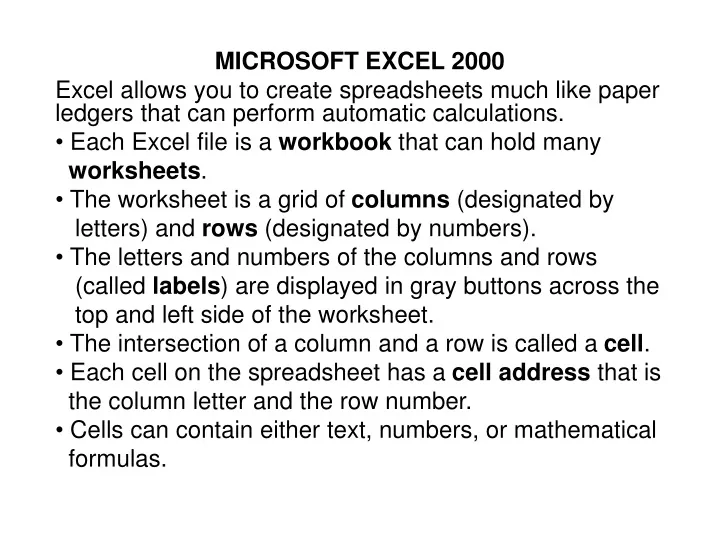
MICROSOFT EXCEL 2000 Excel allows you to create spreadsheets much like paper ledgers that can perform automatic calculations. Each Excel file is a workbook that can hold many worksheets. The worksheet is a grid of columns (designated by letters) and rows (designated by numbers). The letters and numbers of the columns and rows (called labels) are displayed in gray buttons across the top and left side of the worksheet. The intersection of a column and a row is called a cell. Each cell on the spreadsheet has a cell address that is the column letter and the row number. Cells can contain either text, numbers, or mathematical formulas.
Adding and Renaming Worksheets • The worksheets in a workbook are accessible by clicking the worksheet tabs just above the status bar. By default, three worksheets are included in each workbook. • To add a sheet, select Insert|Worksheet from the menu bar. • To rename the worksheet tab, right-click on the tab with the mouse and select Rename from the shortcut menu. Type the new name and press the ENTER key.
The Standard Toolbar This toolbar is located just below the menu bar at the top of the screen and allows you to quickly access basic Excel commands.
New - Select File|New from the menu bar, press CTRL+N, or click the New button to create a new workbook.Open - Click File|Open from the menu bar, press CTRL+O, or click the Open folder button to open an existing workbook.Save - The first time you save a workbook, select File|Save As and name the file. After the file is named click File|Save, CTRL+S, or the Save button on the standard toolbar.Print - Click the Print button to print the worksheet.Print Preview - This feature will allow you to preview the worksheet before it prints.Spell Check - Use the spell checker to correct spelling errors on the worksheet.Cut, Copy, Paste, and Format Painter - These actions are explained in the Modifying A Worksheet section.Undo and Redo - Click the backward Undo arrow to cancel the last action you performed, whether it be entering data into a cell, formatting a cell, entering a function, etc. Click the forward Redo arrow to cancel the undo action.Insert Hyperlink - To insert a hyperlink to a web site on the Internet, type the text into a cell you want to be the link that can be clicked with the mouse. Then, click the Insert Hyperlink button and enter the web address you want the text to link to and click OK.Autosum, Function Wizard, and Sorting - These features are discussed in detail in the Functions tutorial.Zoom - To change the size that the worksheet appears on the screen, choose a different percentage from the Zoom menu.
Moving Through CellsUse the mouse to select a cell you want to begin adding data to and use the keyboard strokes listed in the table below to move through the cells of a worksheet. Movement Key stroke One cell up up arrow key One cell down down arrow key or ENTER One cell left left arrow key One cell right right arrow key or TAB Top of the worksheet(cell A1) CTRL+HOME End of the worksheet (last cell containing data) CTRL+END End of the row CTRL+right arrow key End of the column CTRL+down arrow key Any cell File|Go To menu barcommand
Adding Worksheets, Rows, and Columns • Worksheets - Add a worksheet to a workbook Insert|Worksheet from the menu bar. • Row - To add a row to a worksheet Insert|Rows from the menu bar, or highlight the row by clicking on the row label, right-click with the mouse, and choose Insert. • Column - Add a column Insert|Columns from the menu bar, or highlight the column by click on the column label, right-click with the mouse, and choose Insert.
Resizing Rows and Columns • Resize a row by dragging the line below the label of the row you would like to resize. Resize a column in a similar manner by dragging the line to the right of the label corresponding to the column you want to resize.- OR - • Click the row or column label and select Format|Row|Height or Format|Column|Width from the menu bar to enter a numerical value for the height of the row or width of the column.
Selecting CellsBefore a cell can be modified or formatted, it must first be selected (highlighted). Refer to the table below for selecting groups of cells. Cells to select Mouse action One cell click once in the cell Entire row click the row label Entire column click the column label Entire worksheet click the whole sheet button Cluster of cells drag mouse over the cells or hold down the SHIFT key while using the arrow keys
Moving and Copying Cells • Moving Cells To cut cell contents that will be moved to another cell select Edit|Cut from the menu bar or click the Cut button on the standard toolbar. • Copying Cells To copy the cell contents, select Edit|Copy from the menu bar or click the Copy button on the standard toolbar. • Pasting Cut and Copied Cells Highlight the cell you want to paste the cut or copied content into and select Edit|Paste from the menu bar or click the Paste button on the standard toolbar. • Drag and DropIf you are moving the cell contents only a short distance, the drag-and-drop method may be easier. Simply drag the highlighted border of the selected cell to the destination cell with the mouse.
Freeze Panes If you have a large worksheet with column and row headings, those headings will disappear as the worksheet is scrolled. By using the Freeze Panes feature, the headings can be visible at all times.
Click the label of the row below the row that should remain frozen at the top of the worksheet. • Select Window|Freeze Panes from the menu bar. • To remove the frozen panes, select Window|Unfreeze Panes.
Formatting Toolbar • The contents of a highlighted cell can be formatted in many ways. • Font and cell attributes can be added from shortcut buttons on the formatting bar. • If this toolbar is not already visible on the screen, select View|Toolbars|Formatting from the menu bar.
Format Cells Dialog Box • For a complete list of formatting options, right-click on the highlighted cells and choose Format Cells from the shortcut menu or select Format|Cells from the menu bar.
Number tab - The data type can be selected from the options on this tab. Select General if the cell contains text and number, or another numerical category if the cell is a number that will be included in functions or formulas. • Alignment tab - These options allow you to change the position and alignment of the data with the cell. • Font tab - All of the font attributes are displayed in this tab including font face, size, style, and effects. • Border and Pattern tabs - These tabs allow you to add borders, shading, and background colors to a cell.
Dates and Times • If you enter the date "January 1, 2001" into a cell on the worksheet, Excel will automatically recognize the text as a date and change the format to "1-Jan-01". • To change the date format, select the Number tab from the Format Cells window. • Select "Date" from the Category box and choose the format for the date from the Type box. If the field is a time, select "Time" from the Category box and select the type in the right box. Date and time combinations are also listed. Press OK when finished.
AutoFormatExcel has many preset table formatting options. Add these styles by following these steps: • Highlight the cells that will be formatted.
Select Format|AutoFormat from the menu bar. • On the AutoFormat dialog box, select the format you want to apply to the table by clicking on it with the mouse. Use the scroll bar to view all of the formats available
Click the Options... button to select the elements that the formatting will apply to. Click OK when finished
Formulas • Formulas are entered in the worksheet cell and must begin with an equal sign "=". • The formula then includes the addresses of the cells whose values will be manipulated with appropriate operands placed in between. • After the formula is typed into the cell, the calculation executes immediately and the formula itself is visible in the formula bar. • See the example below to view the formula for calculating the sub total for a number of textbooks. The formula multiplies the quantity and price of each textbook and adds the subtotal for each book.
Linking Worksheets • You may want to use the value from a cell in another worksheet within the same workbook in a formula. • For example, the value of cell A1 in the current worksheet and cell A2 in the second worksheet can be added using the format "sheetname!celladdress". • The formula for this example would be "=A1+Sheet2!A2" where the value of cell A1 in the current worksheet is added to the value of cell A2 in the worksheet named "Sheet2".
Relative, Absolute, and Mixed Referencing • Calling cells by just their column and row labels (such as "A1") is called relative referencing. • When a formula contains relative referencing and it is copied from one cell to another, Excel does not create an exact copy of the formula. • It will change cell addresses relative to the row and column they are moved to. For example, if a simple addition formula in cell C1 "=(A1+B1)" is copied to cell C2, the formula would change to "=(A2+B2)" to reflect the new row. To prevent this change, cells must be called by absolute referencing and this is accomplished by placing dollar signs "$" within the cell addresses in the formula. • Continuing the previous example, the formula in cell C1 would read "=($A$1+$B$1)" if the value of cell C2 should be the sum of cells A1 and B1. Both the column and row of both cells are absolute and will not change when copied. • Mixed referencing can also be used where only the row OR column fixed. For example, in the formula "=(A$1+$B2)", the row of cell A1 is fixed and the column of cell B2 is fixed.
Basic Functions • Functions can be a more efficient way of performing mathematical operations than formulas. • For example, if you wanted to add the values of cells D1 through D10, you would type the formula "=D1+D2+D3+D4+D5+D6+D7+D8+D9+D10". • A shorter way would be to use the SUM function and simply type "=SUM(D1:D10)". Several other functions and examples are given in the table below
Function Example Description SUM =SUM(A1:100) finds the sum of cells A1 through A100 AVERAGE =AVERAGE(B1:B10)finds the average of cells B1 through B10 MAX =MAX(C1:C100) returns the highest number from cells C1 through C100 MIN =MIN(D1:D100) returns the lowest number from cells D1 through D100 SQRT =SQRT(D10) finds the square root of the value in cell D10 TODAY =TODAY()returns the current date (leave the parentheses empty)