Download
1 / 23
230 likes | 240 Vues
Aftershock Relaxation for Japanese and Sumatra Earthquakes. Kazu Z. Nanjo 1 , B. Enescu 2 , R. Shcherbakov 3 , D.L. Turcotte 3 , T. Iwata 1 , & Y. Ogata 1 1, ISM, Tokyo, Japan 2, Kyoto Univ., Kyoto, Japan 3, UC Davis, CA, USA.

E N D
Aftershock Relaxation for Japanese and Sumatra Earthquakes Kazu Z. Nanjo1, B. Enescu2, R. Shcherbakov3, D.L. Turcotte3, T. Iwata1, & Y. Ogata1 1, ISM, Tokyo, Japan 2, Kyoto Univ., Kyoto, Japan 3, UC Davis, CA, USA
Objective: Analyze the decay of the aftershock activity for Japanese and Sumatra earthquakes, using catalogs maintained by Japan Meteorological Agency and Advanced National Seismic System. Approach: Generalized Omori’s law proposed by Shcherbakov et al. (2004, 2005).
The Gutenberg-Richter (GR) law (Gutenberg and Richter, 1954) • N: # of earthq. with mag. ≥ m • A and b: constants • The modified Bath’s law (Shcherbakov and Turcotte, 2004) Δm* = mms - m* m*: mag. of the inferred largest aftershock (m* = A/b) or mag. at the intercept between an extrapolation of the applicable GR law and N=1 mms: main shock mag.
The GR law can be rewritten for aftershocks as • The modified Omori’s law (Utsu, 1962) • dN/dt: rate of occurrence of aftershocks with mag. ≥m • t: time since the main shock • c and τ: characteristic times • p: exponent
Requirement among the parameters • Assume: • p is a constant independent of m and mms (Utsu, 1962) • b, mms, and Δm* are known parameters • Three possible hypotheses: • c is a constant c = c0 andτis dependent on m • τis a constant τ= τ0 and c is dependent on m • c and τ are dependent on m (Shcherbakov et al., 2004, 2005)
Hypoth. I, c = c0 • Hypoth. II, τ = τ0 • Hypoth. III, c and τ are dependent of m • c(m*): the characteristic time; β: a constant • Hypoth. III Hypoth. I if c(m*) = c0 and β = b • Hypoth. II if c(m*) = τ0(p-1) and β= bp
Spatial distribution and GR lawfor Kobe t (days) < 1000 A=4.85, b=0.78 m*=A/b=6.2 ( Mag. ≥ 2 t (days) < 1000 Δm*=1.1 mms=7.3 L (km) = 0.02 X 100.5m_ms [Kagan, 2002]
Aftershock relaxation for Kobe and small aftershocks in the early periods t (days) < 1000 0.01 ≤t < 0.1 0.1 ≤t < 1.0
How to find the best hypothesis • To find the optimal fitting of the prediction to the data for individual hypotheses • Point process modeling with max. likelihood (e.g., Ogata, 1983). • AIC (Akaike, 1974) to find the best hypothesis. AIC = -2(max. log-likelihood) + 2(# of parameters) • # of parameters • Hypoth. I: two (c0 and p) • Hypoth. II: two (τ0 and p) • Hypoth. III: three (c(m*), β, and p)
Test of the generalized Omori’s law for Kobe Hypoth. I, c = c0 Hypoth. II, τ=τ0 AIC=-3376.95 AIC=-3405.00 AIC=-3403.00 Hypoth. III, c and τare dependent on m
Aftershocks of Sumatra earthq. Mag. ≥ 4.5 t (days) < 251 t (days) < 251 A=8.88 b=1.20 m*=A/b=7.4 Δm*=1.6 ( mms=9.0
Test of the generalized Omori’s law for Sumatra Hypoth. I Hypoth. II AIC=-925.42 AIC=-936.76 Hypoth. III AIC=-934.76
Test of the generalized Omori’s law for Tottori Hypoth. I Hypoth. II AIC=-6630.54 AIC=-6654.70 Hypoth. III AIC=-6658.58
Establishment of the GR law (1) Kobe earthq. Hypoth. II c values for different m At time t = 0, dN/dt = 1/τ0 mms=7.3, b=0.78, Δm*=1.1 p=1.16, τ0=0.000508 (days)
Establishment of the GR law (2) Kobe t (days) < 1000, b=0.78 0.1 ≤t < 1.0, b=0.72 0.01 ≤t < 0.1, b=0.79
Establishment of the GR law (2) Kobe t (days) < 1000, b=0.78 0.1 ≤t < 1.0, b=0.72 0.01 ≤t < 0.1, b=0.79 Sumatra t (days) < 251, b=1.20 10 ≤t < 100, b=1.37 1.0 ≤t < 10, b=1.14 0.1 ≤t < 1.0, b=1.27 0.01 ≤t < 0.1, b=1.44
Conclusion • The generalized Omori’s law proposes: • Hypoth. I: τ scales with a lower cutoff mag. m and c is a constant. • Hypoth. II: c scales with m andτ is a constant. • Hypoth. III: Both c and τ scale with m. • 6 main shocks in Japan and Sumatra. • Earthq. catalogs of JMA and ANSS. • AIC and maximum likelihood to find the best hypoth. • The hypoth. II is best applicable to the entire sequence for different cutoff mag. from a state defined immediately after the main shock. • The c value is the characteristic time associated with the establishment of the GR law.
Test of the generalized Omori’s law for Niigata Hypoth. I Hypoth. II AIC=-7151.79 AIC=-7169.11 Hypoth. III AIC=-7167.16
Summary of parameter values m* = A/b Δm* = mms- masmax Δm* = mms- m*
Hypothesis I, c = c0 • Hypothesis II, τ = τ0 • Hypothesis III, c and τ are dependent of m (Shcherbakov et al., 2004, 2005) • c(m*): the characteristic time; β: a constant
Outline • Introduction of the generalized Omori’s law • 6 main shocks considered in this study • 5 Japanese earthquakes • 1 Sumatra earthquake • Application of the law to these earthquakes • Methods to find optimal fitting to the observed aftershock decay • Examples of the application • Summary of the application • Discussion • Conclusion