Download
1 / 54
570 likes | 793 Vues
Analysis of Stray Light in a Brewer Spectrophotometer. Brewers are not Perfect!. C. A. McLinden, D. I. Wardle, C. T. McElroy, &V. Savastiouk Environment Canada. Stolen Stuff:. David Wardle – many slides Tom Grajnar and Mike Brohart – data Volodya Savastiouk – many calculations…

E N D
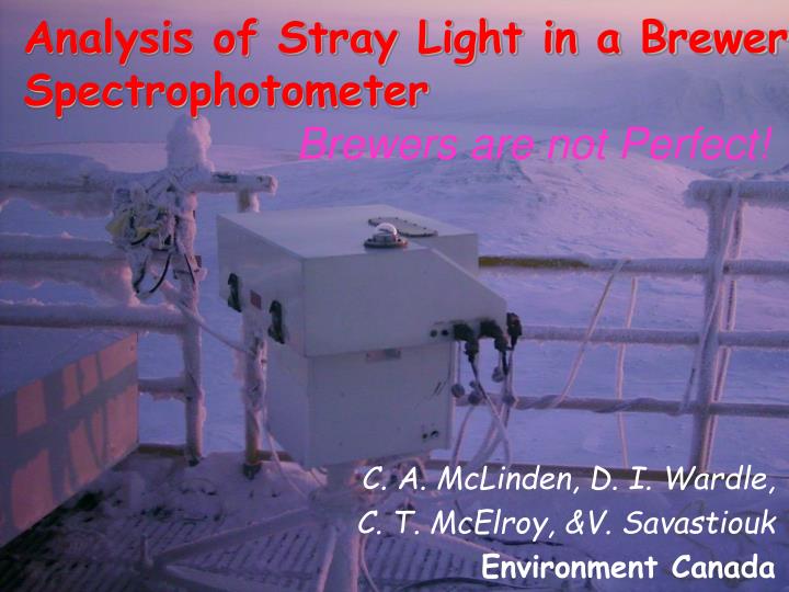
Analysis of Stray Light in a Brewer Spectrophotometer Brewers are not Perfect! C. A. McLinden, D. I. Wardle, C. T. McElroy, &V. Savastiouk Environment Canada
Stolen Stuff: • David Wardle – many slides • Tom Grajnar and Mike Brohart – data • Volodya Savastiouk – many calculations… • Jim Kerr – much code • Chris McLinden - models Brewer Workshop Beijing, China
Brewer Map Brewer Workshop Beijing, China
MSC Toronto Brewer Workshop Beijing, China
Mauna Loa Observatory Brewer Workshop Beijing, China
EurekaWeather Station Brewer Workshop Beijing, China
rationale Global column ozone: Develop confidence in prediction of the future (ozone); models are tuned to reproduce currently measured amounts, also to reproduce measured values during past 20 years. Target accuracy 1.0% 2-sigma. (or maybe 2 or 3 DU) Reasonable to have 20-50? instruments deployed over the world using the measurements with those from space instruments. Over the last 20 years we have almost achieved 1.0% RMS for daily average measurements with our best 3 instruments in Toronto. Brewer Workshop Beijing, China
Dispersion and spectral purity… • Given that we are to measure ozone from • its UV spectrum, we need to know: • accurately the wavelengths of the measurement; in fact • if the wavelength uncertainty is less than 0.01nm it is ok. • if >0.02nm, it is a problem. • Thus we need δλ/λ ~ 1/30,000. • (b) that the much stronger radiation at longer wavelengths • is not interfering with the measurement. Brewer Workshop Beijing, China
Spectrometer • The idea is to have monochromatic light at the exit slit • Diffraction grating is used to separate different wavelengths and send them at different angles Brewer Workshop Beijing, China
The Brewer spectrophotometer optics UV-vis Diffraction grating: 1800 lines/mm 1st order: visible 570-650 nm 2nd order: UV 285-325 nm Also: 1200 and 3600 lines/mm turned by stepper motor Brewer Workshop Beijing, China
Spectrometer layout Brewer Workshop Beijing, China
Spectrometer Gratings and “Marks” Brewer gratings all have the same dispersion in the UV determined by n/d = 3600 lines per mm * order Usually as follows: ---- order in ----- Grating pitch Blazed for UV BLUE RED Mark II S 1800 620 nm 2 Mark V S 1800 620 nm 2 1 Mark IV S 1200 1000 nm 3 2 Mark III D 3600 330 nm 1 Mark VI S 3600 330 nm 1 measuring: ozone NO2 ozone at low sun Mark III is a double spectrometer (D); roughly the same transmission characteristics as the singles (S), except for “stray light”. Another variation is that earlier Brewers have a much smaller Slit#0 . Brewer Workshop Beijing, China
Some dogma……………… For a single wavelength input to a linear spectrometer we can write Signal = intensity of input * f( , s) where is the wavelength of the input radiation & s is the wavelength setting. f( , s) is a response function (count rate. W-1. m2) note: the dispersion function is s = G( steps ) We often do a line scan in which we use a constant input , and vary the setting s. What is more relevant is changing the input given a constant setting. We’ve looked principally at two types of line scan file, c. 9000 from spectral lamps, c. 200 from HeCd Lasers. Brewer Workshop Beijing, China
Dogma continued……………… For a spectrum of input radiation: Signal(s) = P() * f( , s) * d Where P() is the spectral irradiance (watts m-2 nm-1) Most spectrometer users assume the above can be simplified to: Signal(s) = P()*R(s)*q( - s)*d R may be called the responsivity and q the “slit function,” and q() normalized to 1. i.e.: q() d == 1.0 …..Not entirely correct. Brewer Workshop Beijing, China
Slit #0 “slit function” Brewer Workshop Beijing, China
How do Brewers Compare?? Note the log scale! Brewer Workshop Beijing, China
Class I Single Brewers Brewer Workshop Beijing, China
Class II Single Brewers Brewer Workshop Beijing, China
Cass I SB - #017 Brewer Workshop Beijing, China
Class I - #s 007, 017, 109 Brewer Workshop Beijing, China
Extended Scan Singles #s 007, 109 Brewer Workshop Beijing, China
Three Single Brewers – 012, 014, 015 #014, #015 Are Toronto TRIAD Instruments Brewer Workshop Beijing, China
Double Brewers Note: #085 scan was done before the replacement of the ground quartz Brewer Workshop Beijing, China
Double Brewers using 353nm Secondary peak at 325 nm is from impurity of the 353 nm laser Brewer Workshop Beijing, China
325 & 352 nm laser scans …. Brewer Workshop Beijing, China
325 & shifted 353 laser scans… Brewer Workshop Beijing, China
325 & 353 nm comments……… So yes the shape is the same, or is it? Actually the centre is ~10% narrower as the optics dictate has ~10% less energy wings are ~20% lower have ~20% less energy The reasoning is that the ratio of good to bad should be constant regardless of slit width, assuming the aberration-and-diffraction- determined width is smaller than the geometrical (slit-size- determined) width, which appears to be the case. Brewer Workshop Beijing, China
The data Brewer Workshop Beijing, China
How to do laser scans • Need to do at least at two neutral density filter wheel positions to capture both the peak and the “stray light” • It looks like we can use laser scans to find neutral density factors for the single instruments, but not for the doubles. • Need to characterize the ND filters separately for the doubles Brewer Workshop Beijing, China
How to do laser scans • Important: there must be no changes in the optical configuration or laser position when doing multiple ND filters Brewer Workshop Beijing, China
Conclusion • We are learning a great deal about the Brewers with laser scans • We need to help Tom and Mike with establishing rules on how to do laser scans in the field • We also need to propagate this information to the rest of the Brewer community Brewer Workshop Beijing, China
Ozone in Toronto - #s 085, 039 Brewer Workshop Beijing, China
Ozone at Sodankyla Brewer Workshop Beijing, China
Airmass Dependence …in the presence of an ETC error x = ( Fo - F ) / ( alpha * mu ) …with dFo the error in ETC… x’ = ( Fo + dFo - F ) / ( alpha * mu ) = x - dFo / ( alpha * mu ) %x = x - [ x + dFo / ( alpha * mu ) ] / x * 100 = - dFo / ( alpha * mu ) / x * 100 let sx = mu * x slant column ozone %x = %x( mu = 1 ) / mu So at 2400 DU more we expect a 1%(mu = 0) to be 1% / 6 = 0.15% (mu=6) This is NOT what was happening in Sodankyla! Brewer Workshop Beijing, China
Stray LightCorrection Brewer Workshop Beijing, China
Courtesy A. Cede Brewer Workshop Beijing, China
CPFM on WB-57F Brewer Workshop Beijing, China
CPFMStray LightFunction Composition and Photodissociative Flux Measurement Brewer Workshop Beijing, China
Laserscans Single-Brewer stray light rejection is 10-5-10-4 as measured by scanning 325 nm HeCd laserline Instrument function core, FWHM=0.55 nm Stray light shoulder Stray light wing Brewer Workshop Beijing, China
Nature of Stray Light Effect 6 F = Σ al log[ Il ] l=3 X = ( Fo – F ) / ( Δαμ ) Stray light adds signal at each wavelength. largely from longer wavelengths (spectrum gradient) Assume that the stray light is from the longest wavelength, and affects the shortest the most… Brewer Workshop Beijing, China
Stray Light Simplified Brewer ozone is based on slit positions l = 3 to l = 6 Sum over l = 4 to 6 β is stray light fraction F = a3 log[ I3 + βI6 ] + Σ al log[ Il ] F = a3 log[ I3 ( 1+ βI6/ I3 ) ] + Σ al log[ Il ] F = Σ al log[ Il ] + a3 log[ 1+ βI6/ I3 ] = F’ + a3 log[ 1+ βI6/ I3 ] ~ F’ + ζ I6/ I3 with ζ=a3β Now X = ( Fo - F ) / ( Δα * μ ) l = 4 to l = 6 l = 3 to l = 6 Where F’ is the true ozone ratio Brewer Workshop Beijing, China
Rearranging X = ( Fo - F ) / ( Δα * μ ) X = [ Fo – ( F’ + ζ I5 / I2) ] / (Δαμ ) = X’ - ζ I5 / I3 / ( Δαμ ) Now I3 = Io3 exp( - μα3 X’ ) X = X’ - ζ I5 * exp( μα3 X’ ) / Io2 / ( Δαμ ) For μα3 X’ small and I5 only lightly attenuated: X ~ X’ - ζ Io5 * (μα3 X’ + (μα3 X’)2/2 ) / Io3 / (Δαμ ) X ~ X’ - ζ Io5/Io3 X’ - ζ Io5/Io3 μα3 X’2/2 since Δα ~ α3 X ~ X’ ( 1 - ζ Io5/Io3 - ζ Io5/Io3 μα3 X’/2 ) Let ξ = ζα3 / 2 and recognize that Io5 ~ Io3 X ~ X’ ( 1 - ζ - ξμ X’ ) X’ is the true ozone Brewer Workshop Beijing, China
Stray LightCorrection Brewer Workshop Beijing, China
Stray light is modelled by • Calculating transmitted solar irradiances from 290-350 nm at 0.05 nm resolution, multiplying by measured responsitivity, and convolving with laser scan to get synthetic Brewer measurements for each slit • Deriving ETC by performing Langley on synthetic data • Applying Brewer algorithm to synthetic data and ETC • Stray light errors are determined by • Modeling Brewer column including stray light • Modeling Brewer column including only instrument function core • Calculating fractional difference, (xstray – xcore) / xcore Brewer Workshop Beijing, China
Modelled Fractional Stray Light Signal for Brewer #014 • Multiple latitudes and months (ozone profiles), SZAs considered • (which is why there is some scatter) Slit # Brewer Workshop Beijing, China
Comparing Modelled Signals with Observations from Brewer #007 (Fairbanks, May 5, 2001) • compare log(Si)-log(S5), where Si is signal at slit i • Small differences may remain due to assumed Rayleigh, solar flux, slit widths; slit 0 and 1 suggest slightly too much stray light in model i=4 i=3 i=2 i=1 i=0 Brewer Workshop Beijing, China
Modelled Stray light Error in Ozone Columns Error () here caused primarily by stray light wing; thus (009)>(014) Brewer Workshop Beijing, China
Modelled Stray light Error in Ozone Columns ** Model predicts non-zero error even for small slant columns Error () here caused primarily by stray light shoulder; thus (014)>(009) Brewer Workshop Beijing, China
Modelled Stray light Error • Non-zero error at small x is at 1-1.5% level • Jim Kerr (personal communication) estimated this to be about at ~1% error by analyzing Brewer measurements • A small model-measurement inconsistency may remain Brewer Workshop Beijing, China
Parameterizing Laserscans Fitting a Lorentzian to the shoulder region and a constant to the wings seems reasonable (3 parameters) #015 Brewer Workshop Beijing, China