Download
1 / 33
330 likes | 527 Vues
Probability Review. CSE591 – Mobile Computing Georgios Varsamopoulos. Presentation Outline. Basic probability review Important distributions Markov Chains & Random Walks Poison Process Queuing Systems. Basic Probability concepts. Basic Probability concepts and terms.

E N D
Probability Review CSE591 – Mobile ComputingGeorgios Varsamopoulos
Presentation Outline • Basic probability review • Important distributions • Markov Chains & Random Walks • Poison Process • Queuing Systems
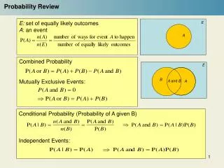
Basic Probability concepts and terms • Basic concepts by example: dice rolling • (Intuitively) coin tossing and dice rolling are Stochastic Processes • The outcome of a dice rolling is an Event • The values of the outcomes can be expressed as a Random Variable, which assumes a new value with each event. • The likelihood of an event (or instance) of a random variable is expressed as a real number in [0,1]. • Dice: Random variable • instances or values: 1,2,3,4,5,6 • Events: Dice=1, Dice=2, Dice=3, Dice=4, Dice=5, Dice=6 • Pr{Dice=1}=0.1666 • Pr{Dice=2}=0.1666 • The outcome of the dice is independent of any previous rolls (given that the constitution of the dice is not altered)
Basic Probability Properties • The sum of probabilities of all possible values of a random variable is exactly 1. • Pr{Coin=HEADS}+Pr{Coin=TAILS} = 1 • The probability of the union of two events of the same variable is the sum of the separate probabilities of the events • Pr{ Dice=1 Dice=2 } = Pr{Dice=1}+{Dice=2} = 1/3
Properties of two or more random variables • The tossing of two or more coins (such that each does not touch any of the other(s) ) simulateously is called (statistically) independent processes (so are the related variables and events). • The probability of the intersection of two or more independent events is the product of the separate probabilities: • Pr{ Coin1=HEADS Coin2=HEADS } =Pr{ Coin1=HEADS} Pr{Coin2=HEADS}
Conditional Probabilities • The likelihood of an event can change if the knowledge and occurrence of another event exists. • Notation: • Usually we use conditional probabilities like this:
Conditional Probability Example • Problem statement (Dice picking): • There are 3 identical sacks with colored dice. Sack A has 1 red and 4 green dice, sack B has 2 red and 3 green dice and sack C has 3 red and 2 green dice. We choose 1 sack randomly and pull a dice while blind-folded. What is the probability that we chose a red dice? • Thinking: • If we pick sack A, there is 0.2 probability that we get a red dice • If we pick sack B, there is 0.4 probability that we get a red dice • If we pick sack C, there is 0.6 probability that we get a red dice • For each sack, there is 0.333 probability that we choose that sack • Result ( R stands for “picking red”):
Moments and expected values • mth moment: • Expected value is the 1st moment: X =E[X] • mth central moment: • 2nd central moment is called variance (Var[X],X)
Geometric Distribution • Based on random variables that can have 2 outcomes (A and A): Pr{A}, Pr{A}=1-Pr{A} • Expresses the probability of number of trials needed to obtain the event A. • Example: what is the probability that we need k dice rolls in order to obtain a 6? • Formula: (for the dice example, p=1/6)
Geometric distribution example • A wireless network protocol uses a stop-and-wait transmission policy. Each packet has a probability pE of being corrupted or lost. • What is the probability that the protocol will need 3 transmissions to send a packet successfully? • Solution: 3 transmissions is 2 failures and 1 success, therefore: • What is the average number of transmissions needed per packet?
Binomial Distribution • Expresses the probability of some events occurring out of a larger set of events • Example: we roll the dice n times. What is the probability that we get k 6’s? • Formula: (for the dice example, p=1/6)
Binomial Distribution Example • Every packet has n bits. There is a probability pΒthat a bit gets corrupted. • What is the probability that a packet has exactly 1 corrupted bit? • What is the probability that a packet is not corrupted? • What is the probability that a packet is corrupted?
The Markov Process • Discrete time Markov Chain: is a process that changes states at discrete times (steps). Each change in the state is an event. • The probability of the next state depends solely on the current state, and not on any of the past states: Pr{Xn+1=j|Xo=io, X1=i1, …, Xn=in} = Pr{Xn+1=j| Xn=in}
Transition Matrix • Putting all the transition probabilities together, we get a transition probability matrix: • The sum of probabilities across each row has to be 1.
Stationary Probabilities • We denote Pn,n+1 as P(n). If for each step n the transition probability matrix does not change, then we denote all matrices P(n) as P. • The transition probabilities after 2 steps are given by PP=P2; transition probabilities after 3 steps by P3, etc. • Usually, limnPn exists, and shows the probabilities of being in a state after a really long period of time. • Stationary probabilities are independent of the initial state
Numeric Example • No matter where you start, after a long period of time, the probability of being in a state will not depend on your initial state.
r r r 1 1 q q q 1 2 3 4 5 p p p Markov Random Walk • A Random Walk Is a subcase of Markov chains. • The transition probabilitymatrix looks like this:
Markov Random Walk • Hitting probability (gambler’s ruin) ui=Pr{XT=0|Xo=i} • Mean hitting time (soujourn time) vi=E[T|Xo=k]
A D Example Problem • A mouse walks equally likely in the following maze • Once it reaches room D, it finds food and stays there indefinitely. • What is the probability that it reaches room D within 5 steps, starting in A? • Is there a probability it will never reach room D?
0.01 0.99 LOW HIGH 0.9 0.1 Example Problem 2 • A variable bit rate (VBR) audio stream follows a bursty traffic model described by the following two-state Markov chain: • In the LOW state it has a CBR of 50Kbps and in the HIGH it has a CBR of 150Kbps. • What is the average bit-rate of the stream?
Example Problem 2 (cont’d) • We find the stationary probabilities • Using the stationary probabilities we find the average bitrate:
Continuous Distributions • Continuous Distributions have: • Probability Density function • Distribution function:
Continuous Distributions • Normal Distribution: • Uniform Distribution: • Exponential Distribution:
Poisson Distribution • Poisson Distribution is the limit of Binomial when n and p 0, while the product np is constant. In such a case, assessing or using the probability of a specific event makes little sense, yet it makes sense to use the “rate” of occurrence (λ=np). • Example: if the average number of falling stars observed every night is λ then what is the probability that we observe k stars fall in a night? • Formula:
Poisson Distribution Example • In a bank branch, a rechargeable Bluetooth device sends a “ping” packet to a computer every time a customer enters the door. • Customers arrive with Poisson distribution of customers per day. • The Bluetooth device has a battery capacity of m Joules. Every packet takes n Joules, therefore the device can send u=m/n packets before it runs out of battery. • Assuming that the device starts fully charged in the morning, what is the probability that it runs out of energy by the end of the day?
Poisson Process • It is an extension to the Poisson distribution in time • It expresses the number of events in a period of time given the rate of occurrence. • Formula • A Poisson process with parameter has expected value and variance . • The time intervals between two events of a Poisson process have an exponential distribution (with mean 1/).
Poisson dist. example problem • An interrupt service unit takes to sec to service an interrupt before it can accept a new one. Interrupt arrivals follow a Poisson process with an average of interrupts/sec. • What is the probability that an interrupt is lost? • An interrupt is lost if 2 or more interrupts arrive within a period of to sec.