Download
1 / 46
460 likes | 465 Vues
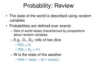
Probability Review. CS479/679 Pattern Recognition Dr. George Bebis. Why Bother About Probabilities?. Accounting for uncertainty is a crucial component in decision making (e.g., classification) because of ambiguity in our measurements.

E N D
Probability Review CS479/679 Pattern RecognitionDr. George Bebis
Why Bother About Probabilities? • Accounting for uncertainty is a crucial component in decision making (e.g., classification) because of ambiguity in our measurements. • Probability theory is the proper mechanism for accounting for uncertainty. • Take into account a-priori knowledge, for example: "If the fish was caught in the Atlantic ocean, then it is more likely to be salmon than sea-bass
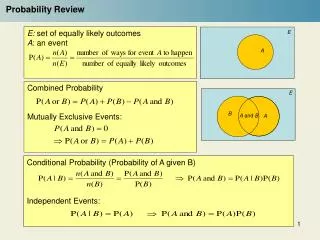
Definitions • Random experiment • An experiment whose result is not certain in advance (e.g., throwing a die) • Outcome • The result of a random experiment • Sample space • The set of all possible outcomes (e.g., {1,2,3,4,5,6}) • Event • A subset of the sample space (e.g., obtain an odd number in the experiment of throwing a die = {1,3,5})
Formulation of Probability • Intuitively, the probability of an event αcould be defined as: • Assumes that all outcomes are equally likely (Laplacian definition) where N(a) is the number of times that eventαhappens in n trials
Axioms of Probability S A1 A3 A2 A4 C)
Unconditional (Prior) Probability • This is the probability of an event in the absence of any evidence. P(Cavity)=0.1 means that “in the absence of any other information, there is a 10% chance that the patient is having a cavity”.
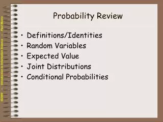
Conditional (Posterior) Probability • This is the probability of an event given some evidence. P(Cavity/Toothache)=0.8 means that “there is an 80% chance that the patient is having a cavity given that he is having a toothache”
Conditional (Posterior) Probability (cont’d) • Conditional probabilities are defined as follows: • The above definitions lead to the chain rule: P(A,B) = P(A/B)P(B) = P(B/A)P(A)
Law of Total Probability • If A1, A2, …, An is a partition of mutually exclusive events and B is any event, then: • Special case : S A1 A3 A2 A4
Bayes’ Rule • Using the definition of conditional probabilities leads to the Bayes’ rule: where:
General Form of Bayes’ Rule • If A1, A2, …, An is a partition of mutually exclusive events and B is any event, then the Bayes’ rule is given by: where
Example • Consider the probability of Disease given Symptom: where:
Example (cont’d) • Meningitis causes a stiff neck 50% of the time. • A patient comes in with a stiff neck – what is the probability that he has meningitis? where P(S/M)=0.5 • Need to know: • The prior probability of a patient having meningitis (P(M)=1/50,000) • The prior probability of a patient having a stiff neck (P(S)=1/20) so, P(M/S)=0.0002
Independence • Two events A and B are independent iff: P(A,B)=P(A)P(B) • Using independence, we can show that: P(A/B)=P(A) and P(B/A)=P(B) • A and B are conditionally independent given C iff: P(A/B,C)=P(A/C)
Random Variables • A random variable (r.v.) is a function that assigns a value to the outcome of a random experiment. X(j)
Random Variables - Example • In an opinion poll, we ask 50 people whether agree or disagree with a certain issue. • Suppose we record a "1" for agree and "0" for disagree. • The sample space for this experiment has 250 elements. • Suppose we are only interested in the number of people who agree. • Define the variable X=number of "1“ 's recorded out of 50. • The new sample space has only 51 elements.
Random Variables (cont’d) • How do we compute probabilities using random variables? • Suppose the sample space is S=<s1, s2, …, sn> • Suppose the range of the random variable Xis <x1,x2,…,xm> • We observe X=xjiff the outcome of the random experiment is an such that X(sj)=xj
Example • Consider the experiment of throwing a pair of dice:
Discrete/Continuous Random Variables • A random variable (r.v.) can be: • Discrete: assumes only discrete values. • Continuous: assumes continuous values (e.g., sensor readings). • Random variables can be described by: • Probability mass/density function (pmf/pdf) • Probability distribution function (PDF)
Probability mass function (pmf) • The pmf of a discrete r.v. X assigns a probability to each possible value x of X. • Notation:given two r.v.'s, X and Y, their pmf are denoted as pX(x) and pY(y); for convenience, we will drop the subscripts and denote them as p(x) and p(y). However, keep in mind that these functions are different!
Probability density function (pdf) • The pdf of a continuous r.v. X shows the probability of being “close” to some number x. • Notation:given two r.v.'s, X and Y, their pdf are denoted as pX(x) and pY(y); for convenience, we will drop the subscripts and denote them as p(x) and p(y). However, keep in mind that these functions are different!
Probability Distribution Function (PDF) • Definition: • Properties of PDF: • (1) • (2) F(x) is non-decreasing
Probability Distribution Function (PDF) (cont’d) • If X is discrete, its PDF can be computed as follows: • If X is continuous, its PDF can be computed as follows:
Probability Distribution Function (PDF) (cont’d) • The pdf can be obtained from the PDF using:
Joint pmf (discrete case) • For n random variables, the jointpmf assigns a probability for each possible combination of values: p(x1,x2,…,xn)=P(X1=x1, X2=x2, …, Xn=xn) Notation:the joint pmf /pdf of the r.v.'s X1, X2, ..., Xn and Y1, Y2, ..., Yn are denoted as pX1X2...Xn(x1,x2,...,xn) and pY1Y2...Yn(y1,y2,...,yn); for convenience, we will drop the subscripts and denote them p(x1,x2,...,xn) and p(y1,y2,...,yn), keep in mind, however, that these are two different functions.
Joint pmf (discrete case) (cont’d) • Specifying the joint pmf requires a large number of values • kn assuming n random variables where each one can assume one of k discrete values. P(Cavity, Toothache) is a 2 x 2 matrix Joint Probability Sum of probabilities = 1.0
Joint pdf (continuous r.v.) For n random variables, the jointpdf gives the probability of being “close” to a given combination of values:
Conditional pdf • The conditionalpdf is defined as follows: • Using the definition of conditional pdfs, leads to the chain rule: • General case:
Independence • Knowledge about independence between r.v.'s is very useful because it simplifies calculations! e.g., if X and Y are independent, then: 2D 1D
Marginalization • Given the joint pmf/pdf, we can compute the pmf/pdf of any subset of variables using marginalization: • Examples:
Normal (Gaussian) Distribution - 1-dimensional: d-dimensional: d x 1 d x d symmetric matrix
Normal (Gaussian) Distribution (cont’d) • Parameters and shape of Gaussian distribution • Number of parameters is • Location determined by μ; shape determined by Σ
Normal (Gaussian) Distribution (cont’d) • Mahalanobis distance: • If the variables are independent, the multivariate normal distribution becomes: Σ is diagonal
Expected Value • The expected value for a discrete r.v. is given by: • The expected value for a continuous r.v. is given by:
Expected Value (cont’d) • In practice, we can approximate E(X) by the sample mean: • The sample mean and expected value are related by:
Variance and Standard Deviation - In practice, we can approximate Var(X) by the sample variance:
Covariance – 2 variables - In practice, we can approximate Cov(X,Y) by the sample covariance:
Covariance Matrix – 2 variables Σ = and Cov(X,Y)=Cov(Y,X) (i.e., symmetric matrix)
Covariance Matrix – n variables (i.e., symmetric matrix) - In practice, we can approximate CX by the sample covariance matrix
Covariance Matrix Decomposition where Φ-1= ΦT
Linear Transformations of random variables Uncorrelated!
Linear Transformations (cont’d) Whitening transform