Skew T Log P Diagram

1. Skew T Log P Diagram AOS 330 LAB 7

2. Review • Difference between ( or dx), and • Hypsometric Equation • Equal Area Transformation

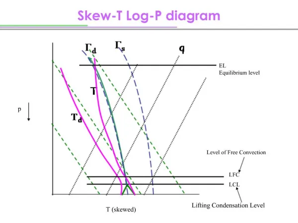
3. 3 Desirable Characteristics of a thermodynamic diagram • They are designed so that area on the diagrams is proportional to energy. • The fundamental lines are straight and thus easy to use. • On a skew-T log P diagram the isotherms(T) are at almost 90o to the isentropes (q). We want the isentropes and isotherms to be far apart to help us to see small temperature changes relative to the dry lapse rate , which is important in determining stability.

4. Atmospheric Soundings Plotted on Skew-T Log P Diagrams • Allow us to identify stability of a layer • Allow us to identify various air masses • Tell us about the moisture in a layer • Help us to identify clouds • Allow us to speculate on processes occurring

5. What are all these lines?

6. Isobars and Isotherms

7. Dry Adiabats and Isotherms

8. Dry Adiabatic Lapse Rate • The rate which T decreases with height for a dry parcel that rises adiabatically. 2 km 12.4 deg. C Adiabatic ascent or descent 1 km 22.2 deg. C 0 km 30 deg. C

9. Pseudoadiabats and Saturated Mixing Ratio lines

10. Hey, what are Pseudoadiabats? To make certain calculations easier, we assume that condensate falls from the parcel as soon as it forms. This obviously isn’t entirely realistic, but the resulting lapse rate only differs from the moist adiabatic rate by about 1% in most instances. Now, let’s see what adiabatic and pseudoadiabatic processes look like when we plot them up.

11. An Adiabatic Process Is this process reversible?

12. Adiabatic / Pseudoadiabatic process Td T Now, is this process reversible?

13. Common Inversions • Subsidence Inversion - typically form in regions of large scale sinking motion (under the subtropical highs, under the left entrance / right exit region of jets) or on the periphery of convective cells. • Radiation Inversion - where would you expect a radiation inversion to develop? and when? • Frontal Inversion - transition zone in between the cold and warm airmass.

14. Subsidence Inversion Suppose air from 200 – 300hPa layer is subsiding adiabatically. 300-200hPa: Lapse rate >0 500 hPa: Close to isothermal Below 500hPa: Stronger and stronger inversions 1000-900hPa: almost 10degC warmer above

15. Subsidence Inversion Potter and Coleman, 2003a

16. Radiation Inversion

17. Radiation Inversion Potter and Coleman, 2003a

18. Frontal Inversion Potter and Coleman, 2003a

19. The Tropopause The last item we’ll be concerned with for today is the tropopause, since it’s the upper limit of what we ordinarily consider “weather.” Is this always the case? There are other important reasons for knowing where the tropopause is that we’ll get to later in the course. There’s a long, technical definition given by the WMO, but in general the tropopause is identified by an abrupt change in lapse rate toward more stable (sometimes even inverted) conditions.

20. Finding the Tropopause

21. References • Hess, 1959: Introduction to Theoretical Meteorology, Holt, Rinehart and Winston, 1959 • Petty, G (2008). A First Course in Atmospheric Thermodynamics, Sundog Publishing. • Potter and Coleman, 2003a: Handbook of Weather, Climate and Water: Dynamics, Climate, Physical Meteorology, Weather Systems and Measurements, Wiley, 2003