Download
1 / 28
350 likes | 748 Vues
Soundings and the Skew-T. Outline. A brief review of static stability The skew-T / log-P Inversions Mixed Layers Air masses, briefly. Adiabatic Process. An adiabatic process is one in which no heat or mass is exchanged with the environment -- in other words,

E N D
Outline • A brief review of static stability • The skew-T / log-P • Inversions • Mixed Layers • Air masses, briefly
Adiabatic Process An adiabatic process is one in which no heat or mass is exchanged with the environment -- in other words, a parcel stays a parcel. In the atmosphere, a parcel expanding / being compressed adiabatically cools / warms at a constant rate with respect to height. The rate at which this happens is known as the dry adiabatic lapse rate, which we’ll denote as gamma: Γd = g / cp ~ 10K / km (Note: Γd is positive, because we define the lapse rate as a rate of cooling for expanding parcels. Don’t let this confuse you!)
Moist Adiabatic Process Now, we know that as a parcel cools, it may reach saturation. When this occurs, the dry adiabatic lapse rate is no longer valid, since further cooling is mitigated by heat released during condensation. The process is now moist adiabatic and the lapse rate is: Γm ~ 6K / km In a few minutes, we’ll see what this looks like on the Skew - T, but first let’s get to the formal definition of static stability.
Static Stability Let Γ = - dT / dz represent the lapse rate in a layer of the atmosphere, we can then define the layer as: 1. Absolutely Stable if Γ < Γm 2. Conditionally Unstable if Γd > Γ > Γm 3. Absolutely Unstable if Γ > Γd Additionally, we define a special case of absolute stability if Γ < 0 (i.e. temperature actually increases with height.) What do we call this?
The Skew-t… • What are each of the lines A-E???
isotherms and adiabats are at right angles to one another,isotherms slope upward to the right, adiabats upward to the left Pseudoadiabats/Moist adiabats curve upward, mixing ratio lines slope upward to the right at an angle to the isotherms
Hey, what are Pseudoadiabats? To make certain calculations easier, we assume that condensate falls from the parcel as soon as it forms. This obviously isn’t entirely realistic, but the resulting lapse rate only differs from the moist adiabatic rate by about 1% in most instances. Now, let’s see what adiabatic and pseudoadiabatic processes look like when we plot them up.
Adiabatic / Pseudoadiabatic Process Now, is this process reversible? Examples…
2 common inversions • Subsidence Inversions • typically form in regions of large scale sinking motion (under the subtropical highs, under the left entrance / right exit region of jets) or on the periphery of convective cells. • Radiation Inversions • where would you expect a radiation inversion to develop? and when?
Mixed Layers A mixed layer is produced by turbulence, which tends to mix conservative tracers such as potential temperature and momentum. Moisture is also mixed, although it may not be mixed uniformly (often there may be a slight decrease with height). The most common mixed layer in the atmosphere is the planetary boundary layer (PBL), which normally occupies the lower kilometer or two of the atmosphere. This feature is normally most well-defined in the late Afternoon. In fact, at other times of day, it may not be mixed at all.
The Elevated Mixed Layer Another type of mixed layer that we’ll be interested in is the elevated mixed layer. This feature typically forms over high terrain (the Rockies, the Mexican Plateau) during the spring and summer. It is VERY important in the severe weather process (it provides a “cap” to the boundary layer) and you’ll no doubt be hearing a lot about it later in the course.
Not all layers are mixed.... ...and if they’re not, they’re known as “stratified layers.” We usually think of stratified layers as those in which the potential temperature and moisture have significant vertical gradients (i.e. they cut across adiabats and mixing ratio lines at high angles). Let’s take a look at a sounding which depicts these features.
Layers and Layers and Layers What suggests a layer of cloud between 650 and 750 mb?
Air Masses We can also identify air masses from sounding data. We do this by looking for features characteristic of certain environments. For example, in arctic regions we generally see persistent radiational cooling, especially in local winter (Why?) This often produces a very deep radiation inversion that can extend from the surface to 700mb or so. Very cold surface temperature and a deep isothermal or inverted surface layer characterizes the arctic air mass, as we see in the next slide.
Now, let’s go to the other extreme. The Tropics! In particular, the tropical oceans and embedded landmasses. The tropical maritime air mass is typified by the following: 1. A warm, moist boundary layer 2. A subsidence inversion in the mid levels (usually around 700mb). 3. An approximately psuedoadiabatic lapse rate over a deep layer We see a typical sounding in the following slide.
What might we expect to see in the tropics from time to time? And for that matter, what about in the midwest during severe weather season? Yep, thunderstorms! Thunderstorms are often called “deep convection” and a hallmark of deep convection is a pseudoadiatic temperature profile over the depth of the troposphere (or nearly so) and near saturation conditions throughout. Note these features in the following slide.
Now Leaving the Troposphere,We hope You enjoyed your Flight! The last item we’ll be concerned with for today is the tropopause, since it’s the upper limit of what we ordinarily consider “weather.” Is this always the case? There are other important reasons for knowing where the tropopause is that we’ll get to later in the course. There’s a long, technical definition given by the WMO, but in general the tropopause is identified by an abrupt change in lapse rate toward more stable (sometimes even inverted) conditions.
Something to Consider Remember that the sounding (and thus the data plotted on the Skew - T) is a snapshot in time and in space. The atmosphere is a fluid and is constantly evolving. Mixed layers, for example, may not always have a “textbook” appearance. By using your knowledge of how and where (and even when) certain features form, you are in a much better position to glean information from a sounding and gain a better understanding of what’s happening in the atmosphere.
Stability Quiz 2 3 4 1