Download
1 / 35
370 likes | 567 Vues
Pattern Formation in Reaction-Diffusion Systems in Microemulsions. Irving R. Epstein Brandeis University with thanks to Vladimir K. Vanag Lingfa Yang http://hopf.chem.brandeis.edu. Patterns in BZ-AOT Microemulsions. Introduction and Motivation Properties of AOT and microemulsions

E N D
Pattern Formation in Reaction-Diffusion Systems in Microemulsions Irving R. Epstein Brandeis University with thanks to Vladimir K. Vanag Lingfa Yang http://hopf.chem.brandeis.edu
Patterns in BZ-AOT Microemulsions • Introduction and Motivation • Properties of AOT and microemulsions • The BZ-AOT system • Experimental results • Localized patterns - mechanism and simulations
BZ-AOT References • V.K. Vanag and IRE, “Inwardly Rotating Spiral Waves in a Reaction-Diffusion System,” Science 294, 835 (2001). • VKV & IRE, "Pattern Formation in a Tunable Reaction-Diffusion Medium: The BZ Reaction in an Aerosol OT Microemulsion," PRL 87, 228301 (2001). • VKV & IRE, “Packet Waves in a Reaction-Diffusion System,” PRL 88, 088303 (2002). • VKV & IRE, “Dash-waves in a Reaction Diffusion System,” PRL 90, 098301 (2003).
Belousov- Zhabotinsky Reaction • Discovered (accidentally) and developed in the Soviet Union in the 50’s and 60‘s • Bromate + metal ion (e.g., Ce3+) + organic (e.g., malonic acid) in 1M H2SO4 • Prototype system for nonlinear chemical dynamics – gives temporal oscillation, spatial pattern formation • Zhabotinsky at Brandeis since 1990
Rw Water HBrO3 MA ferroin Aerosol-OT (sodium bis(2-ethylhexyl) sulfosuccinate) Rd AOT reverse micelles orwater-in-oil microemulsion MA = malonic acid Rw = radius of water core Rd = radius of a droplet, w = Rw = 0.17w Rd = 3 - 4 nm fd= volume fraction of dispersed phase (water plus surfactant) Oil = CH3(CH2)nCH3 Initial reactants of the BZ reaction reside in the water core of a micelle
Diffusion coefficientsL. J. Schwartz at al., Langmuir 15, 5461 (1999)
Droplet Size Distribution “old” “new”
Experimental Setup Gasket Windows A small volume of the reactive BZ-AOT mixture was sandwiched between two flat optical windows 50 mm in diameter. The gap between the windows was determined by the thickness h (= 0.1 mm) of an annular Teflon gasket with inner and outer diameters of 20 mm and 47 mm, respectively. The gasket served as the lateral boundary of the thin layer of microemulsion and prevented oil from evaporating.
BZ-AOT PATTERNS Vanag and Epstein, Phys. Rev. Lett. 87, 228301 (2001).
1-arm anti-spiral Vanag and Epstein, Science 294, 835 (2001).
Turing structures Spots Spots and Stripes Frozen waves Labyrinth
Dash-Wave Vanag and Epstein, Phys. Rev. Lett. 90, 098301 (2003).
Some crude estimates • Droplet diameter = 10 nm • V = (4/3)(d/2)3 = 5 x 10-25 M3 = 5 x 10-22 L • 1 zeptoliter = 10-21 L • 1 M = 6 x 10²³ molecules/L • In each droplet, average number of molecules is: 300 at 1 M concentration 0.3 at 1 mM concentration
A Model for BZ-AOT Oregonator A + Y X k1 X + Y 0 k2 A + X 2X + 2Z k3 2X 0 k4 B + Z hY k5 Interfacial Transfer X S kf S X kb and/or Y T kf’ T Y kb’ whereA = HBrO3, X = HBrO2, Y = Br-, Z = ferriin, B = MA+, BrMA, and S = BrO2• in the oil phase.
Key properties of BZ-AOT system • Size and spacing of droplets can be “tuned” by varying water:AOT and water:octane ratios, respectively • BZ chemistry occurs within water droplets • Non-polar species (Br2, BrO2) can diffuse through oil phase • Diffusion of molecules and droplets occurs at very different rates • Initial bimodal distribution of droplet sizes slowly transforms to unimodal
Localized Patterns - Mechanisms • Bistability (subcritical bifurcation) - need way to stabilize zero-velocity front • Periodic forcing • Global negative feedback • Coupled layers
Global Feedback • A control parameter (e.g., illumination intensity, rate constant) in a spatially extended system depends on values of a quantity (e.g., concentration, temperature, electrical potential) over the entire system (e.g., integral or average) .
Global Feedback/Coupling References • V.K. Vanag, L. Yang, M. Dolnik, A.M. Zhabotinsky and I.R. Epstein, “Oscillatory Cluster Patterns in a Homogeneous Chemical System with Global Feedback,” Nature 406, 389-391 (2000). • V.K. Vanag, A.M. Zhabotinsky and I.R. Epstein, “Pattern Formation in the Belousov-Zhabotinsky Reaction with Photochemical Global Feedback,” J. Phys. Chem. A 104, 11566-11577 (2000). • L. Yang, M. Dolnik, A.M. Zhabotinsky and I.R. Epstein, “Oscillatory Clusters in a Model of the Photosensitive Belousov-Zhabotinsky Reaction-Diffusion System with Global Feedback,” Phys. Rev. E 62, 6414-6420 (2000). • V. K. Vanag, A. M. Zhabotinsky and I.R. Epstein,“Oscillatory Clusters in the Periodically Illuminated, Spatially Extended Belousov-Zhabotinsky Reaction,” Phys. Rev. Lett. 86, 552-555 (2001). • H.G. Rotstein, N. Kopell, A. Zhabotinsky and I.R. Epstein, “A Canard Mechanism for Localization in Systems of Globally Coupled Oscillators” SIAM J. App. Math. (2003, in press).
Clusters and Localization Oscillatory clusters consist of sets of domains (clusters) in which the elements in a domain oscillate with the same amplitude and phase. In the simplest case, a system consists of two clusters that oscillate in antiphase; each cluster can occupy multiple fixed, but not necessarily connected, spatial domains. Clusters may be differentiated from standing waves, which they resemble, in that clusters lack a characteristic wavelength. Standing clusters have fixed spatial domains and oscillate periodically in time. Irregular clusters show no periodicity either in space or in time. Localized clusters display periodic oscillations in one part of the medium, while the remainder appears uniform (may oscillate at low amplitude).
Global Feedback - Experimental Setup • I = Imaxsin2[g(Zav-Z)] • Z = [Ru(bpy)33+] • L2 = 450 W Xe arc lamp • Imax = 4.3 mW cm-2 • L1 = analyzer (45 W) • L3 sets initial pattern (150 W)
Global Feedback Modeling -Discrete Version d[Xi]/dt = k1[A][Yi] - k2[Xi] [Yi] + k3[A][Xi] - 2 k4[Xi][Xi] d[Yi]/dt = - k1[A] [Yi] - k2[Xi] [Yi] + f k5[B] [Zi] + gZav d[Zi]/dt = 2 k3[A][Xi] - k5[B] [Zi] where Zav = [Zi]/N, g = feedback strength
Coupled LayersL. Yang and IRE, “Oscillatory Turing Patterns in Reaction-Diffusion Systems with Two Coupled Layers,” PRL 90, 178303 (2003). • Two reactive layers coupled by a nonreactive “interlayer”. • In each reactive layer, kinetics (activator-inhibitor) and diffusion are the same. • Coupling through interlayer occurs either via activator or inhibitor, but not both, therefore no reaction in that layer. • Constraints (e.g., feed concentrations, illumination) may differ for reactive layers.
Coupled Layers – Model x/t = Dx2x + F(x,z) - (1/)(x-r) z/t = Dz2z + G(x,z) r/t = Dr2r + (1/)(x-r) - (1/’)(u-r) u/t = Du2u + F(u,w) - (1/’)(u-r) w/t = Dw2w + G(u,w) Oregonator: F(x,z) = (1/)[x - x2 - fz(x-q)/(x+q)] G(x,z) = x - z Brusselator: F(x,z) = a - (1+b)x + x2y G(x,z) = bx - x2y and ’ describe inter-layer diffusion (coupling)
·Totally 5 stable solutions: a-Tu, s-Tu, anti-Tu, and a pair of a-SS. ·Combinations C52=20. Here are 13 of them. ·1D simulations: size=64, parameters (a,b)=(16,0.55), d=1,s=50, control h. No. Localized structure foreground background 1 s-Tu on a-SS s-Tu a-SS 2 anti-Tu on a-SS anti-Tu a-SS 3 a-SS on mirror a-SS a-SS 4 h=0.575,not single bump a-Tu a-SS 5 s-Tu a-Tu 6 Anti-Tu a-Tu 7 a-Tu a-Tu 8 s-Tu Anti-Tu 9 a-Tu Anti-Tu 10 a-SS Anti-Tu 11 a-Tu s-Tu 12 a-SS s-Tu 13 Anti-Tu s-Tu Stationary Localized Structures in Coupled Layers (1D) a-Tu on a-SS a-SS on s-Tu s-Tu on a-Tu anti-Tu on s-Tu
Localized Structures • Global coupling, e.g., in photosensitive systems, leads to localized clusters, probably via a canard mechanism • Coupling between “layers” can also generate structures of interest. • Microemulsions provide a convenient experimental system that exhibits rich pattern formation and may be thought of as either globally coupled or “multi-layered”.