Download
1 / 44
440 likes | 680 Vues
ECE 342 Solid-State Devices & Circuits 14. CB and CG Amplifiers. Jose E. Schutt-Aine Electrical & Computer Engineering University of Illinois jschutt@emlab.uiuc.edu. Common Gate Amplifier. Substrate is not connected to the source must account for body effect.

E N D
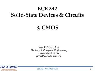
ECE 342 Solid-State Devices & Circuits 14. CB and CG Amplifiers Jose E. Schutt-Aine Electrical & Computer Engineering University of Illinois jschutt@emlab.uiuc.edu
Common Gate Amplifier Substrate is not connected to the source must account for body effect Drain signal current becomes And since Body effect is fully accounted for by using
Common Gate Amplifier Taking ro into account adds a component (RL/Ao) to the input resistance. The open-circuit voltage gain is: The voltage gain of the loaded CG amplifier is:
CG Amplifier as Current Buffer Gis is the short-circuit current gain
High-Frequency Response of CG - Include CL to represent capacitance of load - Cgd is grounded - No Miller effect
High-Frequency Response of CG 2 poles: • fP2 is usually lower than fp1 • fP2 can be dominant • Both fP1 and fP2 are usually much higher than fP in CS case
High-Frequency Analysis of CB Amplifier The amplifier’s upper cutoff frequency will be the lower of these two poles. From current gain analysis
MOS Cascode Amplifier Common source amplifier, followed by common gate stage – G2 is an incremental ground
MOS Cascode Amplifier • CS cacaded with CG Cascode • Very popular configuration • Often considered as a single stage amplifier • Combine high input impedance and large transconductance in CS with current buffering and superior high frequency response of CG • Can be used to achieve equal gain but wider bandwidth than CS • Can be used to achieve higher gain with same GBW as CS
MOS Cascode Analysis KCL at vs2
MOS Cascode Analysis Two cases
MOS Cascode Analysis CASE 1 The voltage gain becomes
MOS Cascode Analysis CASE 2 The voltage gain becomes
MOS Cascode at High Frequency The upper corner frequency of the cascode can be approximated as:
MOS Cascode at High Frequency • Capacitance Cgs1 sees a resistance Rsig • Capacitance Cgd1 sees a resistance Rgd1 • Capacitance (Cdb1+Cgs2) sees resistance Rd1 • Capacitance (CL+Cgd2) sees resistance (RL||Rout)
MOS Cascode at High Frequency If Rsigis large, to extend the bandwidth we must lower RL. This lowers Rd1 and makes the Miller effect insignificant If Rsig is small, there is no Miller effect. A large value of RL will give high gain
Effect of Cascoding (when Rsig=0)
Cascode Example The cascode circuit has a dc drain current of 50 mA for all transistors supplied by current mirror M3. Parameters are gm1=181 mA/V, gm2=195 mA/V, gds1= 5.87 mA/V, gmb2=57.1 mA/V, gds2= 0.939 mA, gds3= 3.76 mA/V, Cdb2 = 9.8 fF, Cgd2 = 1.5 fF, Cdb3=40.9 fF, Cgd3= 4.5 fF. Find midband gain and approximate upper corner frequency The internal conductance of the current source is: Therefore, we use Case 2 to compute the gain
Cascode Example Gain can be approximated by Upper corner frequency is approximated by
BJT Cascode Amplifier Common emitter amplifier, followed by common base stage – Base of Q2 is an incremental ground
BJT Cascode Analysis Ignoring rx2
BJT Cascode Analysis If Rs << rx1+rp1, the voltage gain can be approximated by
BJT Cascode at High Frequency Define rcs as the internal impedance of the current source. R includes generator resistance and base resistance rx1 base of Q1
BJT Cascode at High Frequency There is no Miller multiplication from the input of Q2 (emitter) to the output (collector).
Cascode Amplifier – High Frequency High-frequency incremental model
Cascode Amplifier – High Frequency Applying Kirchoff’s current law to each node: Find solution using a computer
Cascode Amplifier – High Frequency As an example use: gm=0.4 mhos b=100 rp=250 ohms rx=20 ohms Cp=100 pF Cm=5 pf GL=5 mmhos GS’=4.5 mmhos ZEROS POLES sa=8.0 ns-1 sd=-0.0806 nsec-1 sb=-2.02 + j5.99 se=-0.644 sc=-2.02 – j5.99 sf=-4.05 sg=-16.45
Cascode Amplifier – High Frequency If one pole is at a much lower frequency than the zeros and the other poles, (dominant pole) we can approximate w3dB For the same gain, a single stage amplifier would yield: Second stage in cascode increases bandwidth
CE Cascade Amplifier • Exact analysis too tedious use computer • CE cascade has low upper-cutoff frequency
Cascode Amplifier First stage is CE and second stage is CB If Rs << rp1, the voltage gain can be approximated by
Cascode Amplifier – High Frequency High-frequency incremental model
Cascode Amplifier – High Frequency Applying Kirchoff’s current law to each node: Find solution using a computer
Cascode Amplifier – High Frequency As an example use: gm=0.4 mhos b=100 rp=250 ohms rx=20 ohms Cp=100 pF Cm=5 pf GL=5 mmhos GS’=4.5 mmhos ZEROS (nsec-1) POLES (nsec-1) sa=8.0 sd=-0.0806 sb=-2.02 + j5.99 se=-0.644 sc=-2.02 – j5.99 sf=-4.05 sg=-16.45
Cascode Amplifier – High Frequency If one pole is at a much lower frequency than the zeros and the other poles, (dominant pole) we can approximate w3dB For the same gain, a single stage amplifier would yield: Second stage in cascode increases bandwidth