Download
1 / 1
10 likes | 82 Vues
Original image. Reconstruction/ No smoothing. a. b. . . IFT. 4 mm FWHM. 12 mm FWHM. PSWF. IFT. c. e. d. *. *. =. f. =. 619 M-AM. Spatial Smoothing in fMRI using Prolate Spheroidal Wave Functions Martin Lindquist and Tor Wager Department of Statistics, Columbia University

E N D
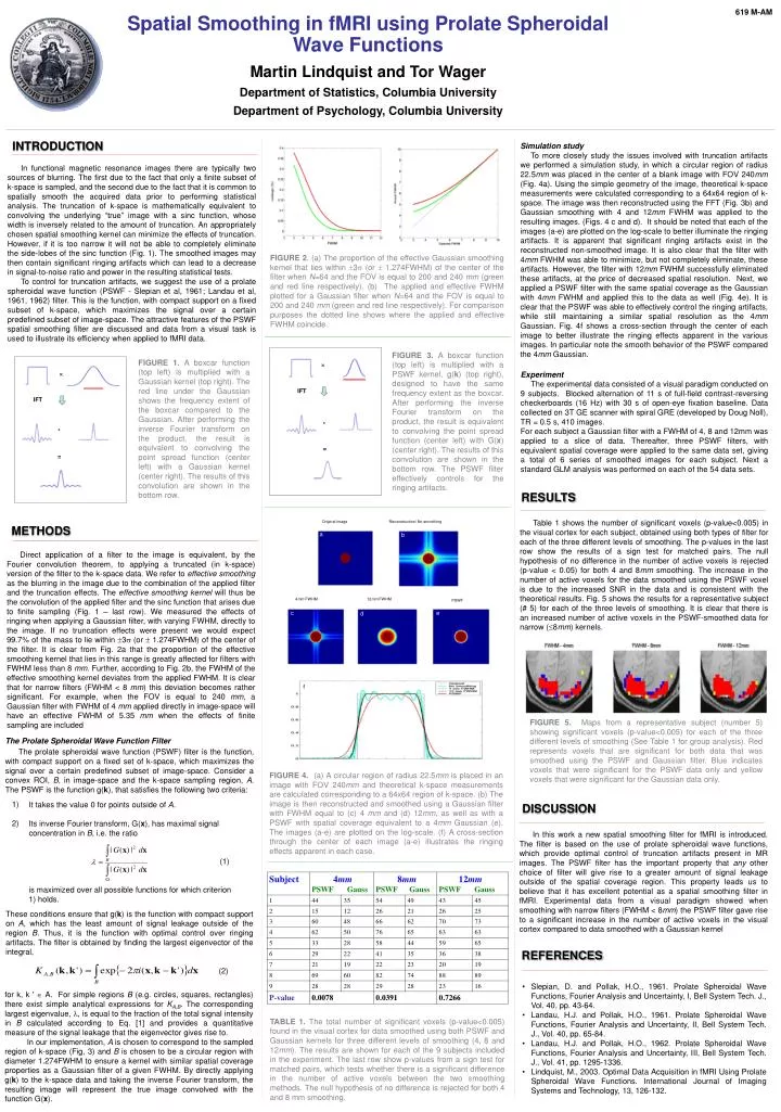
Original image Reconstruction/ No smoothing a b IFT 4mm FWHM 12mm FWHM PSWF IFT c e d * * = f = 619 M-AM Spatial Smoothing in fMRI using Prolate Spheroidal Wave Functions Martin Lindquist and Tor Wager Department of Statistics, Columbia University Department of Psychology, Columbia University INTRODUCTION Simulation study To more closely study the issues involved with truncation artifacts we performed a simulation study, in which a circular region of radius 22.5mm was placed in the center of a blank image with FOV 240mm (Fig. 4a). Using the simple geometry of the image, theoretical k-space measurements were calculated corresponding to a 64x64 region of k-space. The image was then reconstructed using the FFT (Fig. 3b) and Gaussian smoothing with 4 and 12mm FWHM was applied to the resulting images. (Figs. 4 c and d). It should be noted that each of the images (a-e) are plotted on the log-scale to better illuminate the ringing artifacts. It is apparent that significant ringing artifacts exist in the reconstructed non-smoothed image. It is also clear that the filter with 4mm FWHM was able to minimize, but not completely eliminate, these artifacts. However, the filter with 12mm FWHM successfully eliminated these artifacts, at the price of decreased spatial resolution. Next, we applied a PSWF filter with the same spatial coverage as the Gaussian with 4mm FWHM and applied this to the data as well (Fig. 4e). It is clear that the PSWF was able to effectively control the ringing artifacts, while still maintaining a similar spatial resolution as the 4mm Gaussian. Fig. 4f shows a cross-section through the center of each image to better illustrate the ringing effects apparent in the various images. In particular note the smooth behavior of the PSWF compared the 4mm Gaussian. In functional magnetic resonance images there are typically two sources of blurring. The first due to the fact that only a finite subset of k-space is sampled, and the second due to the fact that it is common to spatially smooth the acquired data prior to performing statistical analysis. The truncation of k-space is mathematically equivalent to convolving the underlying “true” image with a sinc function, whose width is inversely related to the amount of truncation. An appropriately chosen spatial smoothing kernel can minimize the effects of truncation. However, if it is too narrow it will not be able to completely eliminate the side-lobes of the sinc function (Fig. 1). The smoothed images may then contain significant ringing artifacts which can lead to a decrease in signal-to-noise ratio and power in the resulting statistical tests. To control for truncation artifacts, we suggest the use of a prolate spheroidal wave function (PSWF - Slepian et al, 1961; Landau et al, 1961, 1962) filter. This is the function, with compact support on a fixed subset of k-space, which maximizes the signal over a certain predefined subset of image-space. The attractive features of the PSWF spatial smoothing filter are discussed and data from a visual task is used to illustrate its efficiency when applied to fMRI data. FIGURE 2. (a) The proportion of the effective Gaussian smoothing kernel that lies within 3 (or 1.274FWHM) of the center of the filter when N=64 and the FOV is equal to 200 and 240 mm (green and red line respectively). (b) The applied and effective FWHM plotted for a Gaussian filter when N=64 and the FOV is equal to 200 and 240 mm (green and red line respectively). For comparison purposes the dotted line shows where the applied and effective FWHM coincide. FIGURE 3. A boxcar function (top left) is multiplied with a PSWF kernel, g(k) (top right), designed to have the same frequency extent as the boxcar. After performing the inverse Fourier transform on the product, the result is equivalent to convolving the point spread function (center left) with G(x) (center right). The results of this convolution are shown in the bottom row. The PSWF filter effectively controls for the ringing artifacts. FIGURE 1. A boxcar function (top left) is multiplied with a Gaussian kernel (top right). The red line under the Gaussian shows the frequency extent of the boxcar compared to the Gaussian. After performing the inverse Fourier transform on the product, the result is equivalent to convolving the point spread function (center left) with a Gaussian kernel (center right). The results of this convolution are shown in the bottom row. Experiment The experimental data consisted of a visual paradigm conducted on 9 subjects. Blocked alternation of 11 s of full-field contrast-reversing checkerboards (16 Hz) with 30 s of open-eye fixation baseline. Data collected on 3T GE scanner with spiral GRE (developed by Doug Noll), TR = 0.5 s, 410 images. For each subject a Gaussian filter with a FWHM of 4, 8 and 12mm was applied to a slice of data. Thereafter, three PSWF filters, with equivalent spatial coverage were applied to the same data set, giving a total of 6 series of smoothed images for each subject. Next a standard GLM analysis was performed on each of the 54 data sets. RESULTS Table 1 shows the number of significant voxels (p-value<0.005) in the visual cortex for each subject, obtained using both types of filter for each of the three different levels of smoothing. The p-values in the last row show the results of a sign test for matched pairs. The null hypothesis of no difference in the number of active voxels is rejected (p-value < 0.05) for both 4 and 8mm smoothing. The increase in the number of active voxels for the data smoothed using the PSWF voxel is due to the increased SNR in the data and is consistent with the theoretical results. Fig. 5 shows the results for a representative subject (# 5) for each of the three levels of smoothing. It is clear that there is an increased number of active voxels in the PSWF-smoothed data for narrow (8mm) kernels. METHODS Direct application of a filter to the image is equivalent, by the Fourier convolution theorem, to applying a truncated (in k-space) version of the filter to the k-space data. We refer to effective smoothing as the blurring in the image due to the combination of the applied filter and the truncation effects. The effective smoothing kernel will thus be the convolution of the applied filter and the sinc function that arises due to finite sampling (Fig. 1 – last row). We measured the effects of ringing when applying a Gaussian filter, with varying FWHM, directly to the image. If no truncation effects were present we would expect 99.7% of the mass to lie within 3 (or 1.274FWHM) of the center of the filter. It is clear from Fig. 2a that the proportion of the effective smoothing kernel that lies in this range is greatly affected for filters with FWHM less than 8 mm. Further, according to Fig. 2b, the FWHM of the effective smoothing kernel deviates from the applied FWHM. It is clear that for narrow filters (FWHM < 8 mm) this deviation becomes rather significant. For example, when the FOV is equal to 240 mm, a Gaussian filter with FWHM of 4 mm applied directly in image-space will have an effective FWHM of 5.35 mm when the effects of finite sampling are included FIGURE 5. Maps from a representative subject (number 5) showing significant voxels (p-value<0.005) for each of the three different levels of smoothing (See Table 1 for group analysis). Red represents voxels that are significant for both data that was smoothed using the PSWF and Gaussian filter. Blue indicates voxels that were significant for the PSWF data only and yellow voxels that were significant for the Gaussian data only. The Prolate Spheroidal Wave Function Filter The prolate spheroidal wave function (PSWF) filter is the function, with compact support on a fixed set of k-space, which maximizes the signal over a certain predefined subset of image-space. Consider a convex ROI, B, in image-space and the k-space sampling region, A. The PSWF is the function g(k), that satisfies the following two criteria: FIGURE 4. (a) A circular region of radius 22.5mm is placed in an image with FOV 240mm and theoretical k-space measurements are calculated corresponding to a 64x64 region of k-space. (b) The image is then reconstructed and smoothed using a Gaussian filter with FWHM equal to (c) 4 mm and (d) 12mm, as well as with a PSWF with spatial coverage equivalent to a 4mm Gaussian (e). The images (a-e) are plotted on the log-scale. (f) A cross-section through the center of each image (a-e) illustrates the ringing effects apparent in each case. 1) 2) It takes the value 0 for points outside of A. Its inverse Fourier transform, G(x), has maximal signal concentration in B, i.e. the ratio (1) is maximized over all possible functions for which criterion 1) holds. DISCUSSION In this work a new spatial smoothing filter for fMRI is introduced. The filter is based on the use of prolate spheroidal wave functions, which provide optimal control of truncation artifacts present in MR images. The PSWF filter has the important property that any other choice of filter will give rise to a greater amount of signal leakage outside of the spatial coverage region. This property leads us to believe that it has excellent potential as a spatial smoothing filter in fMRI. Experimental data from a visual paradigm showed when smoothing with narrow filters (FWHM < 8mm) the PSWF filter gave rise to a significant increase in the number of active voxels in the visual cortex compared to data smoothed with a Gaussian kernel These conditions ensure that g(k) is the function with compact support on A, which has the least amount of signal leakage outside of the region B. Thus, it is the function with optimal control over ringing artifacts. The filter is obtained by finding the largest eigenvector of the integral, (2) REFERENCES • Slepian, D. and Pollak, H.O., 1961. Prolate Spheroidal Wave Functions, Fourier Analysis and Uncertainty, I, Bell System Tech. J., Vol. 40, pp. 43-64. • Landau, H.J. and Pollak, H.O., 1961. Prolate Spheroidal Wave Functions, Fourier Analysis and Uncertainty, II, Bell System Tech. J., Vol. 40, pp. 65-84. • Landau, H.J. and Pollak, H.O., 1962. Prolate Spheroidal Wave Functions, Fourier Analysis and Uncertainty, III, Bell System Tech. J., Vol. 41, pp. 1295-1336. • Lindquist, M., 2003. Optimal Data Acquisition in fMRI Using Prolate Spheroidal Wave Functions. International Journal of Imaging Systems and Technology, 13, 126-132. for k, k ' A. For simple regions B (e.g. circles, squares, rectangles) there exist simple analytical expressions for KA,B. The corresponding largest eigenvalue, , is equal to the fraction of the total signal intensity in B calculated according to Eq. [1] and provides a quantitative measure of the signal leakage that the eigenvector gives rise to. In our implementation, A is chosen to correspond to the sampled region of k-space (Fig, 3) and B is chosen to be a circular region with diameter 1.274FWHM to ensure a kernel with similar spatial coverage properties as a Gaussian filter of a given FWHM. By directly applying g(k) to the k-space data and taking the inverse Fourier transform, the resulting image will represent the true image convolved with the function G(x). TABLE 1. The total number of significant voxels (p-value<0.005) found in the visual cortex for data smoothed using both PSWF and Gaussian kernels for three different levels of smoothing (4, 8 and 12mm). The results are shown for each of the 9 subjects included in the experiment. The last row show p-values from a sign test for matched pairs, which tests whether there is a significant difference in the number of active voxels between the two smoothing methods. The null hypothesis of no difference is rejected for both 4 and 8 mm smoothing.