Download
1 / 19
190 likes | 293 Vues
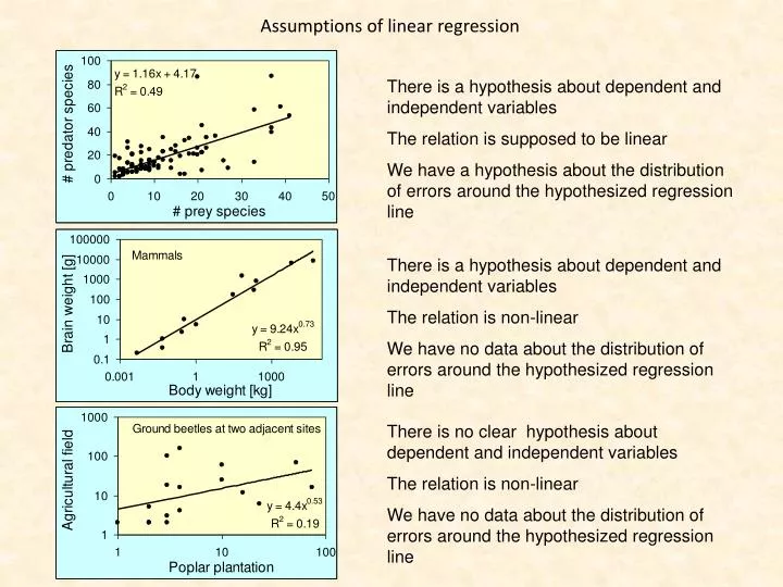
Assumptions of linear regression. There is a hypothesis about dependent and independent variables The relation is supposed to be linear We have a hypothesis about the distribution of errors around the hypothesized regression line.

E N D
Assumptions of linearregression There is a hypothesis about dependent and independent variables The relation is supposed to be linear We have a hypothesis about the distribution of errors around the hypothesized regression line There is a hypothesis about dependent and independent variables The relation is non-linear We have no data about the distribution of errors around the hypothesized regression line There is no clear hypothesis about dependent and independent variables The relation is non-linear We have no data about the distribution of errors around the hypothesized regression line
Assumptions: A linear model applies The x-variable has no error term The distribution of the y errors around the regression line is normal Least squares method
The second example is nonlinear We hypothesize the allometric relation W = aBz Nonlinear regression model Linearised regression model Assumption: The distribution of errors is lognormal Assumption: The distribution of errors is normal
Y=e0.1X+norm(0;Y) Y=X0.5enorm(0;Y) In both cases we have some sort of autocorrelation Using logarithms reduces the effect of autocorrelation and makes the distribution of errors more homogeneous. Non linear estimation instead puts more weight on the larger y-values. If there is no autocorrelation the log-transformation puts more weight on smaller values.
Linearregression European bat species and environmentalcorrelates
N=62 Matrixapproach to linearregression Xis not a squarematrix, henceX-1doesn’texist.
Thespecies – arearelationship of Europeanbats Whataboutthe part of varianceexplained by our model? 1.16: Averagenumber of species per unit area (speciesdensity) 0.24: spatialspeciesturnover
How to interpretthecoefficient of determination Total variance Rest (unexplained) variance Residual (explained) variance Statisticaltestingisdone by an F or a t-test.
The general linear model A model thatassumesthat a dependent variable Y can be expressed by a linearcombination of predictorvariables X iscalled a linear model. ThevectorEcontainstheerrorterms of eachregression. Aimis to minimizeE.
The general linear model Iftheerrors of thepreictorvariablesareGaussiantheerror term e shouldalso be Gaussian and means and variancesareadditive Total variance Explainedvariance Unexplained(rest) variance
Multipleregression Model formulation Estimation of model parameters Estimation of statisticalsignificance
R: correlationmatrix n: number of cases k: number of independent variablesinthe model D<0 isstatistically not significant and should be eliminatedfromthe model. Adjusted R2
Thefinal model Verylowspeciesdensity (log-scale!) Realisticincrease of speciesrichnesswitharea Increase of speciesrichnesswithwinterlength Increase of speciesrichnessathigherlatitudes A peak of speciesrichnessatintermediatelatitudes Isthis model realistic? The model makesrealisticpredictions. Problem mightarise from the intercorrelationbetween the predictorvariables (multicollinearity). We solvethe problem by a step-wiseapproacheliminatingthevariablesthatareeither not significantorgiveunreasonableparametervalues Thevarianceexplanation of thisfinal model ishigherthanthat of theprevious one.
Multiple regression solves systems of intrinsically linear algebraic equations Polynomialregression General additive model • The matrix X’X must not be singular. It est, the variables have to be independent. Otherwise we speak of multicollinearity. Collinearity of r<0.7 are in most cases tolerable. • Multiple regression to be safely applied needs at least 10 times the number of cases than variables in the model. • Statistical inference assumes that errors have a normal distribution around the mean. • The model assumes linear (or algebraic) dependencies. Check first for non-linearities. • Check the distribution of residuals Yexp-Yobs. This distribution should be random. • Check the parameters whether they have realistic values. Multiple regression is a hypothesis testing and not a hypothesis generating technique!!
Standardizedcoefficients of correlation Z-tranformeddistributionshave a mean of 0 an a standard deviation of 1. In thecase of bivariateregression Y = aX+b, Rxx = 1. HenceB=RXY. Hencetheuse of Z-transformedvaluesresultsinstandardizedcorrelationscoefficients, termedb-values