Download
1 / 18
190 likes | 510 Vues
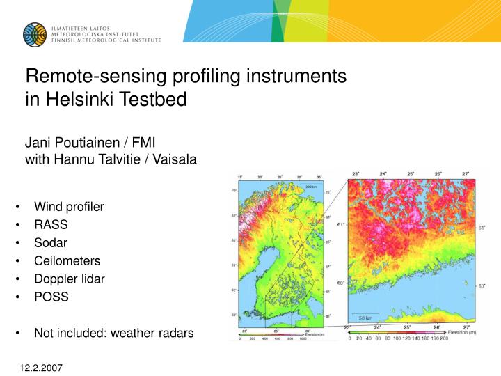
Remote-sensing profiling instruments in Helsinki Testbed Jani Poutiainen / FMI with Hannu Talvitie / Vaisala. Wind profiler RASS Sodar Ceilometers Doppler lidar POSS Not included: weather radars. 12.2.2007. Wind Profiler at Malmi Airport LAP-3000 wind profiler (8/2005-11/2006)

E N D
Remote-sensing profiling instruments in Helsinki TestbedJani Poutiainen / FMIwith Hannu Talvitie / Vaisala • Wind profiler • RASS • Sodar • Ceilometers • Doppler lidar • POSS • Not included: weather radars 12.2.2007
Wind Profiler at Malmi Airport • LAP-3000 wind profiler (8/2005-11/2006) • RASS for virtual temperature profiling (10/2005-11/2006) • Remote access from Vaisala (Boulder and Vantaa) and FMI • Pulse Doppler RAdio Detection And Ranging device • Transmission pulse of electromagnetic energy with target backscattering. • The profiler computes height by using the time interval between transmission of the pulse and reception of the return signal. • Wind speed and direction are obtained with Doppler principle, i.e. wave will shift in frequency because of the motion of the target relative to the observer. • Maximum backscattering power occurs when atmospheric irregularities are about half the size of the radar wavelength (Bragg scatter). – perturbance in refractive index – backscatter from hydrometeors • Local horizontal uniformity of the wind field is assumed. • For detailed info, see: http://testbed.fmi.fi/docs/Profiler-info.html
VAISALA LAP3000 SPECIFICATIONS Operating frequency 1290 MHz Minimum height 75-150m Maximum height 2-5km Range resolution 60, 100, 200, 400m; Testbed configuration 102m Wind speed accuracy <1 m/s Wind direction accuracy <10 ° Averaging time 3-60 minutes RF power output 600 W peak Antenna Electrically steerable micropatch phased-array panels Aperture 2.7 m2 (4 panels) Direction Zenith and ±15,5º from zenith in 4 orthogonal directions Beamwidth ~9º MTBF 40,000 hours Other operating frequencies 915, 920, 924, 1280, 1299, 1357.5 MHz
Approaching low pressure system Sea breeze
Effects on profiler range performance Dependence on atmospheric conditions. Rapid and significant changes. Affecting conditions: humidity, turbulence, precipitation, high winds and temperature. Dependence on ground/sea clutter environment, available radio frequency emission bandwidth, aircrafts and birds. Vertical profiles of mean availability for the wind measurements at various sites (Dibbern et al., 2003)
Radio acoustic sounding system (RASS) • Profiles of virtual temperature, i.e. temperature uncompensated for humidity or pressure. • Continuous acoustic sine wave synchronized to RADAR frequency, about 2.6 kHz (half wavelength). • Acoustic wave acts as an artificial target. • Profiler receives resulting backscatter and effectively measures the speed of sound. • Sound speed is related to air temperature thus temperature information can be calculated. • Profiler gathers wind velocity data for the largest portion of an averaging period and virtual temperature data for the remaining portion. In Testbed configuration, typically 27 min for wind and 3 min for temperature measurement. • Strong winds may transport the acoustic signal away from vertical alignment. • Atmosphere absorbs the acoustic signal, much determined by temperature, humidity and pressure. Frequency 2-3 kHz Minimum height 75-150m Maximum height 1-1.5km Range resolution 60, 100, 200, 400m In Testbed conf: lowest range 149 m, up to 400 ..1500 m, step 62 m Temperature accuracy 1 °C Averaging time 3-60 minutes Sound pressure 1 m above transducer 132 dB Aperture 1.2 m2 (4 sources)
Data examples Approaching cloud deck first warms upper layer (above 250 m) until cooling finally starts with clearing (17:30). At the same time, closer to ground (150-250 m) cooling takes place with northerly winds. Descending inversion
Panu Maijala VTT • Sodar model: REMTECH PA1 • Location at Malmi, 08-11/2006 • Emission of acoustic pulse and detection of echo Doppler frequency shift. Echo signal relates to thermal turbulence in the atmosphere. • Sounds like a bird singing • Linux based measurement system
Ceilometers in the Testbed domain • 7 pcs of CT25K (FMI) • Cloud heights and amounts • 6 pcs of CL31 • Cloud heights, amounts and backscatter profile • Nurmijärvi, Röykkä • Mäntsälä, Purola • Porvoo, Tirmo • Helsinki, Vallila • Vantaa, Vantaanlaakso • Helsinki, Malmi
Lens Receiver Mirror Transmitter Vaisala CL31 Measurement range 0 ... 7.5 km Measurement resolution 10 m or 5 m Reporting interval 2 ... 120 s, selectable Measurement interval 2 s default; 16 s in Testbed configuration Laser source Indium Gallium Arsenide (InGaAs) Diode Laser Center wavelength 910 ± 10 nm at 25 °C Operating Mode Pulsed Nominal pulse properties at full range measurement: Energy 1.2 μWs ± 20% Peak power 11 W typical Width, 50% 110 ns typical Repetition rate 10.0 kHz Average power 12.0 mW Max Irradiance 760 μW/cm² measured with 7 mm aperture Beam divergence ±0.4 mrad x ±0.7 mrad • Measurement of cloud height and amount, or vertical visibility. And backscatter profile. • LIDAR technology (LIDAR = Light detection and ranging). • Laser pulses are sent out in a vertical or near-vertical direction. • The backscatter is caused by haze, fog, mist, virga, precipitation and clouds. • Knowing light speed and time delay between the launch and the detection of signal gives cloud base.
Noora Eresmaa FMI Mixing height estimation and Testbed-data CL31-ceilometers • The 2-step algorithm is under development • An idealized backscattering profile B(z) is fitted to the measured profile by the formula • zSL corresponds to the lower mixing layer (Step1); zML to the upper one (Step2). An example of the ceilometer profile fitting (15 April 2006 at 10:00 UTC in Vallila, Helsinki)
Christoph Münkel Vaisala Ground fog measurement with Vaisala Ceilometer CL31 Strong and clearly structured signal from ground fog patches.
Karen Bozier Univ. of Salford Doppler lidar – University of Salford & Halo photonics • Atmospheric backscatter and vertical wind velocity measurement. Measurements of the eddy dissipation rate and the integral length scale of turbulent eddies. • Construction: optical base unit, the weather-proof antenna and the signal processing and data acquisition unit. • Selectable parameters such as the length of the range gate, maximum range and number of pulses accumulated for each measurement and the spectral resolution. • Investigation of the day-night boundary layer transition. Parameters Description/Value Operating wavelength 1.55 mm Pulse Repetition Frequency 20 kHz Energy per pulse 10 mJ Beam divergence 50 mrad ~ 5cm at 1 km Range gate 30 m Minimum range 30 m Maximum range up to 7 km dependant on atmospheric conditions Temporal resolution 0.1 – 30 s
Karen Bozier Univ. of Salford 9th August 2006 between 10:40 – 11:00 UTC.
The picture above shows modeled distribution of particulate matter concentrations on the August 9th 2006 at 09:00 UTC (source: http://www.fmi.fi/). The unit in the given color scale is µg/m3. The picture below presents ceilometer Vaisala CL31 backscatter profiles at Helsinki Malmi site on the same day (08:57-09:03 UTC).
POSS – Precipitation occurrence sensor system • Järvenpää 12/05- • Malmi 12/05-05/06 • Jokioinen 06/06- • Customs declaration until 11/08, Communications Regulatory Authority permission for extension in process.
Kenneth Wu Met Service Canada • Precipitation detection • Type identification (dominant type): Drizzle ( L), Rain (R), Snow (S), Hail (A), Indeterminate ( P) • Intensity and rate estimation: Very light (-- ), Light ( - ), Moderate ( ), Heavy ( + ) • Rain drop size distribution (DSD) • Doppler shifted frequency is proportional to the velocity component in the boresight of the antenna. • Mean power of the Doppler signal depends on: raindrop size, antenna pattern, transmitter power and window transmission losses. • Both amplitude and frequency from a single particle vary as it passes through the measurement volume. • Microwave (10.525 GHz, 3cm) CW Doppler bi-static radar • 43 mw nominal output power • Measurement range approx. 2 m • Measurement volume 30 m3 • Heated TX/RX window with bird deterrent • Maximum total power consumption: 200W • Operates under all weather conditions