Download
1 / 17
170 likes | 380 Vues
Modeling Permafrost – a CMT component. Elchin Jafarov Vladimir Romanovsky Sergei Marchenko Geophysical Institute University of Alaska Fairbanks Boulder, October, 2011. Frozen Soil (Permafrost). Thawing Permafrost. http://www.libraryindex.com/pages/3372/Permafrost.html

E N D
Modeling Permafrost – a CMT component Elchin Jafarov Vladimir Romanovsky Sergei Marchenko Geophysical Institute University of Alaska Fairbanks Boulder, October, 2011
Thawing Permafrost http://www.libraryindex.com/pages/3372/Permafrost.html http://ipy.arcticportal.org/index.php?/ipy/detail/permafrost/ http://nasadaacs.eos.nasa.gov/articles/2005/2005_permafrost.html
Soil Moisture Soil texture by grain size table Neil Davis “Permafrost”
Active Layer Thickness Ice-nucleation temperature Cryotic Noncryotic Partially Frozen Frozen Unfrozen Water content Unfrozen water content Freezing point depression T < 0oC T > 0oC 0oC C.R. Burn. (1999). The Active Layer: Two Contrasting Definition.
Active Layer Thickness Ice-nucleation temperature Cryotic Noncryotic Partially Frozen Frozen Unfrozen Saturation coeff. Water content Unfrozen water content Freezing point depression T < 0oC T > 0oC 0oC C.R. Burn. (1999). The Active Layer: Two Contrasting Definition.
GIPL2-MPI The GIPL-MPI model schematic diagram. S. Marchenko (2008)
Input Datasets Monthly averaged air temperature (oC) during January 1980 (SNAP). • The GCMs composite was downscaled to 2 by 2 km resolution using knowledge-based system PRISM. Monthly averaged precipitation (mm) during January 1980 (SNAP).
Input Datasets Karlstrom, T.N.V., et al., 1964. Surficial geology of Alaska. U.S. Geol.Surv., Misc. Geol. Inv. Map I-357, scale 1:1,584,000
Results Projections of the decadal average MAGT at 2 m depth
GIPL CMT component GIPL in CMT
Coupling TopoFlow with GIPL2 Topoflow GIPL ET Runoff INF Thawed VWC f/t depth Frozen
Acknowledgments Funding & State of Alaska