Download
1 / 59
590 likes | 718 Vues
“LOGISTICS MODELS” Andrés Weintraub P. Departament Industrial Engineering University of Chile PASI Santiago Agosto 2013. Column Generation Combined with Constraint Programming to Solve a Technician Dispatch Problem. Cristián E. Cortés Civil Engineering Department Andrés Weintraub

E N D
“LOGISTICS MODELS”Andrés Weintraub P.Departament Industrial EngineeringUniversity of ChilePASISantiagoAgosto 2013 IFORS Hawaii, July 2005
Column Generation Combined with Constraint Programming to Solve a Technician Dispatch Problem Cristián E. Cortés Civil Engineering Department Andrés Weintraub Sebastián Souyris Industrial Engineering Department University of Chile Michel Gendrau Ecole Polytechnique, Montreal
Motivation • Real Problem: Dynamic dispatch of technicians of Xerox Chile to repair failures of their machinesalong the day. • The proposed scheme is based upon the classic formulation of the Vehicle Routing Problem with Soft Time Windows (VRPSTW), and it is formulated and solved as a Dantzig-Wolfe decomposition by using column generation along with classical insertion heuristics, under a constraint programming approach. • Xerox strategic objective: Client satisfaction, so technical service becomes relevant
goal response times time Client j calls The Problem: Characteristic • Requests along the day, which must to be served in the same day. • Technicians are specialized in certain type of machines. • Service times are stochastic and depend on the type of machine and the specific failure. • Clients have priority levels
The problem • The objective function for assigning technicians and jobs is to minimize two components: • the sum of the differences between goal response times of clients and the effective service time provided by Xerox • the sum of travel times. IFORS Hawaii, July 2005
Approaches • Based on queuing theory • Dynamic Traveling Salesman Problem (Psaraftis,1988) • Dynamic Traveling Repairman Problem (Bertsimas et. al., 1991) • Algorithmic • Analytical Models • Heuristics and Metaheurstics • Tabu Search (Gendreau et. al., 1999), Ant Colony System (Montemanni, 2002).
Vehicle k arrives to client j Vehicle k idle after serving j Client j calls Vehicle k idle after serving i Model: VRPTW time
:Multi Objective Parameter OF: Minimize TW violation and travel time Each customer must be served Path ends in the final fictitious technician Flow Conservation Temporal and feasibility constraints Nature of Variables
Master Problem Set Partitioning Model COLUMN GENERATOR Sub Problem Reformulation Dual Multipliers Columns Constraint Programming
Description of the General Process • Generate a set of initial routes, feasible problem. • Solve a linear relaxation of the master problem with the generated pool of routes. • 3. From the dual variables associated to the constraints of each machine in the master problem, generate the route with minimum reduced cost (subproblem). If its reduced cost cr*<0 , go to 4, otherwise go to 5. • Using the sub-problem generate all possible columns with reduced cost less than and length L, where is a control parameter that satisfies , thus • . Go to 2. • 5. Solve MP using B&B including all the columns generated in the previous steps, obtaining the final routes to be followed by each technician. IFORS Hawaii, July 2005
Optimal Solution Number of Iterations IP Model v/s CG • Instance: 5 technicians, 20 clients • IP Model: optimal solution in 3.5 hrs. • CG: optimal solution in 15 iterations, 3.7 sec. Model coded with ILOG Concert Technology, and solved by using CPLEX 9.0 and SOLVER 6.0
Example Real Instance • Real Operation: Normal working day, 36 clients,9 technicians • Optimization total time 500 sec. • The following maps show observed routing versus optimized routing.
5 11 30 15 16 4 28 7 22 25 9 26 36 24 10 1 17 12 27 2 18 29 34 8 21 32 19 3 31 33 13 20 35 23 6 14
SP: Shortest Path Problem With Soft Time Windows OF: Minimize reduced cost One technician follow the new path Flow Conservation Path ends in the final fictitious node Temporal and feasibility constraints Nature of Variables
How to solve it? • Dynamic Programming: • The most used approach in literature. • Difficult to implement and solve it under Branch and Price scheme. • Constraint Programming: • Good performance for short routes. • Easy to implement and solve it under Branch and Price scheme with Constraint Branching.
Actual Path 5 11 30 15 16 4 28 7 22 25 9 26 36 24 10 1 17 12 27 29 2 18 34 8 21 32 3 19 31 33 13 20 35 23 6 14
OPT Path 5 11 30 15 16 4 28 7 22 25 9 26 36 24 10 1 17 12 27 2 18 29 34 8 21 32 19 3 31 33 13 20 35 23 6 14
But, this procedure doesn’t assure optimality… • Improve CG methodology: Branch and Price. • Previous methodology does not ensure optimality • When descending along the B&B tree, new routes with negative reduced cost could be found • B&P: Generate columns at each node of the Branch & Bound • Columns generated at each node have to be consistent with the partition associated to such a node • First Approach using Maestro Library for B&P (ILOG). • Same Master Problem. • Sub Problem with IP Shortest Path Model. =>only solves medium instance (40 clients 10 technicians) in prohibited computational time.
Second Approach B&P • Same Master Problem. • Sub Problem with : • Ryan and Foster (1981) Branching Strategy. Wich one is better? • Constraint Programming. • Dynamic Programming. (Shortest Path with Soft Time Windows)
Model is modified, replacing temporal constraints by Stochastic Service Times • SVRP Literature: Formulate the problem either resource or chance constraint, or both. • Robust Optimization: Box of uncertainty: completely independent uncertainty for each si given by a closed, convex and bounded uncertainty set Worst Case: all service times take the upper bound value, which is improbable
Stochastic Service Times Independent service time uncertainty per technician Worst Case: for each route, first clients complete their repair time until Uk (Optimal solution of Robust problem has variations in service times as early as possible, which was analytically proved and it is also a very intuitive result)
Two new Variables: Upper value for client i service time If previous client has max service time Max Service Time above average by technician Max Service Time above average by client Relation between variables x and y Relation between variables z and y Model forces to have repair time of max length at the beginning of each route (worst case).
Characteristic of the problem • Mathematical Model • Decomposition approach • Robust approach • Robust results • Conclusions
Robust Model Test • New constraints are added to the SubProblem. • Test: • Comparison with deterministic model. • Real data. • For each customer, assume Weibell distribution (which represents repair times properly). Parameters for Weibell, derived from data. Obtain 1000 values of repair time for each customer, leading to 1000 simulations. • For each instance we test different values. • Experiments consider sensitivity in standard deviation associated with real data
Characteristic of the problem • Mathematical Model • Decomposition approach • Robust approach • Robust results • Conclusions
Conclusions and Further Research • Robust Model represent quite well the worst case, easy to implement and give better results than determinist model. • Benefits of the robust model strongly depend on the variability of the real data uncertainty. • CP allows to easily implement the Robust model under the same B&P algorithm developed for the deterministic case • Dynamic Routing, Fleet design
If a column is created: • Incorporate constraint: this new column can´t be created again into the subproblem. • Solver Search: • Dichotomic strategic. • Procedure: depth first search. • How many columns must be generated at each iteration? • Under which criteria?
0 4 7 2 9 11 13 1 8 3 5 12 10
0 4 7 2 9 11 13 1 8 3 5 12 10
0 4 7 2 9 11 13 1 8 3 5 12 10
0 4 7 2 9 11 13 1 8 3 5 12 10
0 4 7 2 9 11 13 1 8 3 5 12 10
0 4 7 2 9 11 13 1 8 3 5 12 10
0 4 7 2 9 11 13 1 8 3 5 12 10
0 4 7 2 9 11 13 1 8 3 5 12 10 Feasible Route!
0 4 7 2 9 11 13 1 8 3 5 12 10 Reconstruct the path with this nodes.
0 4 7 2 9 11 13 1 8 3 5 12 10
Master Problem: Then the branching constraints are the clients i and j have to be covered: Left branch by the same column Right branch by different columns Branching Strategy: Constraint Branching (Ryan and Foster) If a basic solution is fractional then there exist two clients i and j such that: because every column must be different.
Branching Strategy: Constraint Branching (Ryan and Foster) Two type of columns Three type of columns j j j j j i i i i i
Ryan and Foster (1981) branching strategy: benefits • All constraints are imposed at the sub-problem directly • B&B terminates after a finite number of branches since there are only a finite number of pairs of rows. • Each branching decision eliminates a large number of variables from consideration .
Example Real Instance • Real Operation: Normal working day, 36 clients,9 technicians • Optimization total time 100 sec. • The following maps show observed routing versus optimized routing.