The Viper Main Interface Layout and interpretation

1. The Viper Main Interface Layout and interpretation

2. The Viper Main Interface Layout and interpretation Selecting predictors and predictands Global month changes

3. The Viper Main Interface Layout and interpretation Selecting predictors and predictands Global month changes Predictors quality, availability Historical statistics

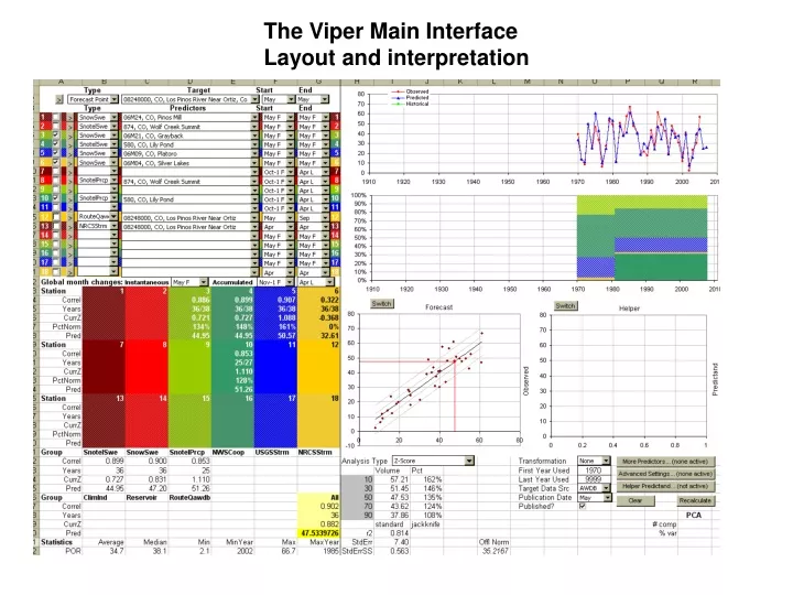
4. The Viper Main Interface Layout and interpretation Selecting predictors and predictands Forecast vs observed time series Station availability, weights Global month changes Predictors quality, availability Historical statistics

5. The Viper Main Interface Layout and interpretation Selecting predictors and predictands Forecast vs observed time series Station availability, weights Global month changes Predictors quality, availability Fcst vs obs scatterplot Helper variable Scatterplot/ Forecast progression Historical statistics

6. The Viper Main Interface Layout and interpretation Selecting predictors and predictands Forecast vs observed time series Station availability, weights Global month changes Predictors quality, availability Fcst vs obs scatterplot Helper variable Scatterplot/ Forecast progression Settings Probability bounds Historical statistics

7. Selecting predictors and predictands Forecast vs observed time series Station availability, weights Global month changes Predictors quality, availability Fcst vs obs scatterplot Helper variable Scatterplot/ Forecast progression Settings Probability bounds Historical statistics The Viper Main Interface Layout and interpretation There’s more if you scroll right: Relate any variable to another

8. Selecting the predictand: Specify a type (e.g. Forecast point, snow, precipitation…)

9. Selecting the predictand: Specify a type (e.g. Forecast point, snow, precipitation…) Specify target station Sorted by USGS ID, upstream to downstream If other than streamflow, ordered alphabetically

10. Selecting the predictand: Specify a type (e.g. Forecast point, snow, precipitation…) Specify target station Sorted by USGS ID, upstream to downstream If other than streamflow, ordered alphabetically Specify months “Jan “ : January of this year “Jan-1” : January of last year “Jan F” : 1st half of January (e.g. Jan 1, Jan1-15) “Jan L” : 2nd half of January (e.g. Jan 16, Jan 16-31)

11. Selecting the predictors: Is the station used or not? (checked = yes)

12. Selecting the predictors: Is the station used or not? (checked = yes) Station groups as defined on “station” sheet

13. Selecting the predictors: Is the station used or not? (checked = yes) Station groups as defined on “station” sheet Clicking on a carat box sends you to the data sheet for that station. Experts may learn how to edit data once there.

14. Predictor quality, availability

15. Predictor quality, availability Station number and status indicator (e.g. low skill, missing) Period of record correlation coefficient with predictand 1=good,0=bad Predictor years (overlapping with target/ total) Realtime value as z-score (+1 high,-1 low) and % period of record normal Realtime forecast as if only one predictor was being used

16. Predictor quality, availability Station number and status indicator (e.g. low skill, missing) Period of record correlation coefficient with predictand 1=good,0=bad Predictor years (overlapping with target/ total) Realtime value as z-score (+1 high,-1 low) and % period of record normal Realtime forecast as if only one predictor was being used

17. Predictor quality, availability Station number and status indicator (e.g. low skill, missing) Period of record correlation coefficient with predictand 1=good,0=bad Predictor years (overlapping with target/ total) Realtime value as z-score (+1 high,-1 low)and % period of record normal Realtime forecast as if only one predictor was being used

18. Some data problems Missing: Realtime data value is unavailable Low skill: The predictor is too poor to be considered (correlation too low) Short por: The predictor does not have enough years in common with the target

19. Group information Correlation and predictions are represented by each station group. “All” is using all stations together. The bold yellow cell is the “bottom line” of the forecast (in k-ac-ft).

20. Historical statistics of target POR – period of record (all years) 71-00 – all available** years from 1971-2000 (official 1971-2000 normal available to right)

21. 1 2 1 Analysis type: Z-Score or PCA regression 2 Probability bound information: (gray is editable) Probability of exceedence (low probability = wet) Volume in thousands of acre-feet Percent of 1971-2000 normal

22. 1 2 3 4 1 Analysis type: Z-Score or PCA regression 2 Probability bound information: (gray is editable) Probability of exceedence (low probability = wet) Volume in thousands of acre-feet Percent of 1971-2000 normal 3 Skill statistics: Correlation^2, Standard Error, Standard Error Skill Score Including all years or jackknifed (leave 1 year out at a time) 4. Official 1971-2000 normal

23. Forecast (blue) versus observed (red) time series and historical forecasts (green)

24. Forecast (blue) versus observed (red) time series and historical forecasts (green)

25. Forecast (blue) versus observed (red) time series and historical forecasts (green) “Forecast” is the calibration set of forecasting equation you set up “Historical forecast” is historical published outlook, issued back in the day Leadtime of historical forecast is specified in cell O46 “Publication Date”

26. R^2 = .33 Station weighting time series For each year, what is the relative contribution of skill (R^2) from each station? Taller means more skillful information Example: 1 station… Contributes 100% of skill in all years

27. .33 R^2 = .44 R^2 = .77 Station weighting time series For each year, what is the relative contribution of skill (R^2) from each station? Taller means more skillful information Example: 1 station… Contributes 100% of skill in all years 3 stations… 1 long, medium and short record These are the weights used in Z-Score regression. Not used in PCA, but shown anyway. (Gets more complicated with multiple groups, but idea the same)

28. Forecast vs observed scatter plot Gray lines show exceedence probabilities Red dot shows current forecast “Toggle graph” identifies individual years

29. Equation output Predictand Published forecasts Helper Helper predictand (x) vs original target (y) Appears blank if helper not used In this example, AWDB vs USGS data shown “Switch” brings you to a plot of forecast vs leadtime

30. 1 2 3 4 1 Do non-linear regression by transforming predictand (e.g. square root) 2 Limit the start and end year of the analysis 3 Acquire predictand flow data from AWDB or USGS 4 Publication date of forecast (changes each month)

31. 1 2 3 4 5 6 1 Do non-linear regression by transforming predictand (e.g. square root) 2 Limit the start and end year of the analysis 3 Acquire predictand flow data from AWDB or USGS 4 Publication date of forecast (changes each month) 5 Buttons to view additional predictors, advanced settings, helper 6 Number of principal components retained and % variance explained

32. Scroll right on main interface “Original” = Value stored in recent data sheet “Estimated” = What you might expect given the other variable “O-E” = Original-Estimated