Download
1 / 15
150 likes | 270 Vues
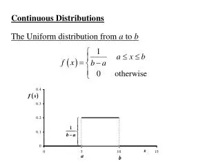
Continuous Distributions. And the Normal Curve. Density curves A density curve is a mathematical model of a distribution. The total area under the curve, by definition , is equal to 1, or 100%.

E N D
Continuous Distributions And the Normal Curve
Density curves A density curve is a mathematical model of a distribution. The total area under the curve, by definition, is equal to 1, or 100%. The area under the curve for a range of values is the proportion of all observations for that range. Histogram of a sample with the smoothed, density curve describing theoretically the population.
The mean of a density curve is the balance point, at which the curve would balance if made of solid material. The median and mean are the same for a symmetric density curve. The mean of a skewed curve is pulled in the direction of the long tail. Median and mean of a density curve The median of a density curve is the equal-areas point, the point that divides the area under the curve in half.
Normal distributions Normal (or Gaussian) distributions are a family of symmetrical, bell shaped density curves defined by a mean μ and a standard deviation σ x x e = 2.71828…
Here means are different (μ= 10, 15, and 20) while standard deviations are the same (σ= 3) The means are the same(μ=15) & the standard deviations are different (σ = 2, 4, and 6).
About 68% of all observations are within 1 standard deviation (σ ) of the mean (μ). About 95% of all observations are within 2 σof the mean. • Almost all (99.7%) observations are within 3 σof the mean. All Normal curves N( μ,σ2) share the same properties Inflection point mean=64.5 standarddeviation=2.5 X ̴N(64.5,2.52)
The standard Normal distribution Because all Normal distributions share the same properties, we can standardize our data to transform any Normal curve N(μ, σ) into the standard Normal curve N(0,1). N(64.5,2.52) ) N(0,1) => Standardized height (no units) For each x we calculate a new value, z (called a z-score).
Standardizing: calculatingz-scores Az-scoremeasuresthenumberof standarddeviationsthatadatavaluex is fromthemean Eg Whenx is 1standard deviationlargerthanthemean,thenz=1 When x is 2 standard deviations below the mean, then z=-2
Using Normal Distribution Curve table This table gives the area under the standard Normal curve to the left of any z value. .0082is the area underN(0,1) left of z=-2.40 0.0069is the area underN(0,1) left ofz= -2.46 .0080is the area underN(0,1) left ofz= -2.41 (…)
Women heights follow the N(64.5”,2.52”) distribution. What percent of women are shorter than 67 inches tall (that’s 5’6”)? N(64.5, 2.52) Area= ??? Area= ??? mean = 64.5" standard deviation = 2.5" x (height) =67"
Percent of women shorter than 67” For z = 1.00, the area under the standard Normal curve to the left of z is 0.8413. Conclusion: 84.13% of women are shorter than 67”. By subtraction, 1 - 0.8413, or 15.87% of women are taller than 67". Area0.84 Area0.16
Area= 0.9901 Method#1:arearightofz=arealeftof-z Area= 0.0099 z= -2.33 BecausetheNormaldistribution is symmetrical,thereare2ways thatyoucancalculatetheareaunder thestandardNormal curvetotherightof az value Method#2: area rightof z = 1- arealeftof z
To calculate the area between 2 z- values, first get the area under N(0,1) to the left for each z-value from Table A. Then subtract the smaller area from the larger area. Tips on using Table A . The area under N(0,1) for a single value of z is zero (Try calculating the area to the left of z minus that same area!) areabetweenz1andz2=arealeft ofz1–arealeft ofz2
TheNationalCollegiateAthleticAssociation(NCAA)requires Division I athletes toscoreatleast 820 on thecombinedmathand verbalSATexam tocompetein theirfirstcollegeyear.TheSATscoresof 2003 were approximately normal with mean1026and standard deviation209. WhatproportionofallstudentswouldbeNCAAqualifiers(SAT "820)?