Download
1 / 14
150 likes | 281 Vues
Voronoi Diagrams for Oriented Spheres. Franz Aurenhammer. Joint work with M. Peternell H. Pottmann J. Wallner. Voronoi Diagram. The classical case …. Size small, easy computation Separators are lines (hyperplanes). Power Diagram.

E N D
Voronoi Diagrams for Oriented Spheres Franz Aurenhammer Joint work with M. Peternell H. Pottmann J. Wallner
Voronoi Diagram The classical case …. Size small, easy computation Separators are lines (hyperplanes) Computational Geometry
Power Diagram Theorem [AI, 1988] Separators are hyperplanes iff the diagram is the power diagram for some set of spheres. Computational Geometry
Quadratic-form Distance T Q(p,q) = (q-p) · M · (q-p), point sites p,q M nonsingular, k x k T T W.l.o.g. M symmetric: Q(p,q) = ½ (q-p) · (M+M ) · (q-p) Separators are hyperplanes Power diagrams are induced Computational Geometry
Examples M = I closest-point Voronoi diagram (Eucl. squared) M = -I farthest-point diagram M = ( ) Q(p,q) is twice the area of rectangle with diagonal pq [CDL] 0 1 1 0 T M = diag (1,…,1,-1) quasi-Euclidean distance Computational Geometry
Oriented Spheres Points in 3D Oriented spheres in 2D Quasi-Eucl. distance d: squared tangent length Principal spheres Computational Geometry
Motivation Special relativity: Events = points in quasi-Euclidean space (pseudo-metric governed by M) Isometric mappings = Lorentz transformations Value of d(p,q) is a Lorentz invariant < 0 time-like (√|d| = life time) > 0 space-like (√d = Euclidean distance) = 0 light-like Computational Geometry
Physical Meaning of d Light cone (d=0) separates time domain (d>0) from space domain (d<0) Computational Geometry
Diagram for d (space ≈ - time) Just a power diagram (for the principal spheres). But: d is not a metric (light-cones) Sidedness may be violated Site extremal region unbounded Computational Geometry
Variant 1 (time ≈ space) Distance D D = |d(p,q)| Two types of separators Structure determined by light cone arrangement Computational Geometry
Variant 2 (space driven) Δ Distance ∞ d(p,q) if ≥ 0 { = Δ ∞ ∞ otherwise Refinement of light cone arrangement Not face-to-face Computational Geometry
Variant 3 (space driven) Δ Distance 0 d(p,q) if > 0 { = Δ 0 0 otherwise Lives in the complement of the union of time domains Face-to-face Computational Geometry
What else AssociatedDelaunay triangulations? Quasi-Euclidean circum-circle…. Computational Geometry
Thank you Computational Geometry