Download
1 / 53
610 likes | 926 Vues
Voronoi diagrams generalizations and applications in VLSI manufacturing. Evanthia Papadopoulou IBM T.J. Watson Research Center Athens University of Economics and Business. Overview. Voronoi diagram – powerful mathematical object Encountered in various application areas

E N D
Voronoi diagrams generalizations and applications in VLSI manufacturing Evanthia Papadopoulou IBM T.J. Watson Research Center Athens University of Economics and Business
Overview • Voronoi diagram – powerful mathematical object • Encountered in various application areas • Our contributions to the theory and application of Voronoi diagrams • VLSI Critical AreaExtraction • Important problem in VLSI yield prediction • Sensitivity of VLSI design to random defects during manufacturing – essential for IC manufacturing • Model and solve using generalizations of Voronoi diagrams • Hausdorff Voronoi diagram • Higher order Voronoi diagrams of segments • IBM-Cadence Voronoi CAA tool for VLSI yield prediction
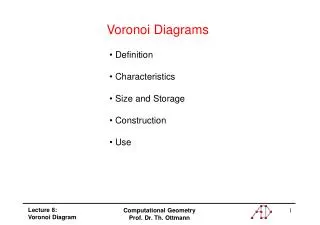
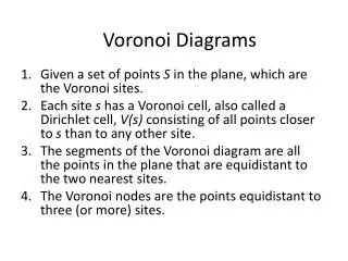
Delauney Triangulation Voronoi diagram for n point-sites in the plane • Voronoi diagram: partitioning into Voronoi regions • Voronoi region of a site s is locus of points closer to s than to any other site • Planar graph: Voronoi edges, Voronoi vertices, Size O(n), n= # sites • Interesting properties • Encodes nearest neighbor information s
Voronoi diagram of segments • Same concept, planar graph, linear size • Voronoi edges (bisectors) consist of line segments and parabolic arcs • Parabolic arcs – robustness issues – harder to use in practice
Voronoi diagram of disks / weighted points • Apollonius graph [http://www.cgal.org]
Medial axis of a polygon : Voronoi diagram • Voronoi diagram in the interior of a polygon is known as medial axis • Sites: edges and vertices of the polygon • Medial axis: skeleton of the polygon
Higher order Voronoi diagrams • kth order Voronoi region: locus of points closest to a k-tuple of sites • Planar graph of size: O(k(n-k)), n = # sites • Encodes k nearest neighbor information • Studied mostly for points [Lee 82, Chazelle & Edelsbrunner 87, Aurenhammer 90] Segments [Papadopoulou ISAAC07]
Farthest Voronoi diagram • Farthest Voronoi region of s: locus of points farther from s than any other site • Unbounded regions only – size O(n), n = # sites • Studied mostly for points [survey Aurenhammer & Klein 00] Segments [Aurenhammer, Drysdale & Krasser 06]
Generalizations of Voronoi diagrams[survey: Aurenhammer & Klein 00] • Higher order and farthest Voronoi diagrams • Different metric (non-euclidean) Voronoi diagrams • Different types of sites • Abstract Voronoi diagrams • Defined in terms of bisecting curves – not sites • Voronoi diagrams in higher dimensions • Limited work • Research in combinatorial/algorithmic aspects but also in implementation, application, and robustness issues
Voronoi Software • Robust implementation efforts are relatively recent • Basics available in CGAL -- Computational Geometry Algorithms Library -- open source project • Site http://www.cgal.org
VLSI Critical Area Analysis • VLSI Yield: Percentage of working chips over all chips manufactured • Very important consideration/limitation in today’s chip manufacturing • Factors of Yield loss: Random defects and Systematic defects • Random defects: dust/contaminants on materials and equipment • Can result in considerable yield loss • Prediction of yield loss due to random defects: Critical Area Analysis • Critical Area: Measure reflecting the sensitivity of a VLSI design to random defects during manufacturing • Essential for IC manufacturing – DFM (design for manufacturing) initiatives under consideration
Open Metal Shorted Metal Examples of faults due to random defects Open Metal Foreign Material Short
Critical Area • Critical Area: A(r) : area where if a defect of radius r is centered causes a circuit failure D(r): density function of the defect size Defect of size r = disk of radius r
A(r) -- shorts for one defect size r r Critical Area
A(r) – open faults for one defect size r(assuming no interconnect loops)(broken shape = open fault) r Critical Area Integral for all defect sizes
Methods to compute Critical Area • Monte Carlo simulation [Initial work at IBM (see e.g. Stapper & Rosner Trans. Semic. Manuf. 95) also Walker & Director CMU 86 (VLASIC)] • Randomly draw large number of defects following D(r) • Check for faults • Oldest most widely implemented technique • Computationally intensive • Shape shifting methods [see e.g. AFFCA –Bubel et al DFT’95 , Allan& Walton TCAD99, Zachariah & Chacravarty TVLSI 00] • Based on shape expansion / shrinking • Many variants • Very expensive to compute A(r) for medium/large r needed in integration • Quadratic number of expanded shape intersections. Repetition for different r • Statistical Layout sampling in combination with shape-shifting techniques [G. Allan TCAD00]
Methods to compute Critical Area2 • The Voronoi method [Papadopoulou and Lee TCAD99, Papadopoulou TCAD01, Papadopoulou Algorithmica 04, Papadopoulou ISAAC07] • Idea: partition layout into regions where critical area integral can be easily computed (analytically) • Critical area computation becomes trivial once appropriate Voronoi diagram derived • Can be combined with layout sampling techniques for fast critical area estimate at chip level [IBM patent filing Papadopoulou et al. 2007] • Developed into the IBM Voronoi CAA tool – (now licenced to Cadence) • used extensively in production by IBM Manufacturing • Claim 60x throughput improvemets over previously used tools [Maynard and Hibbeler ASMC’05]
Critical Area via Voronoi diagrams • Shorts: Ac 2nd order Voronoi diagram of polygons (L∞) [Papadopoulou & Lee T-CAD 99] • Simple Open Faults: Ac Voronoi diagram of (weighted) segments (L∞) [Papadopoulou T-CAD 01] • Via Blocks: Ac Hausdorff Voronoi diagram (L∞) [Papadopoulou T-CAD 01, Algorithmica 04] • General Open Faults: Ac Higher order Voronoi diagram of (weighted) segments (L∞) [Papadopoulou ISAAC 2007] • Analytical Critical Area integration – no error • O(n log n) – type of algorithms in most cases • Critical Area Integral = Summation of simple terms derived from Voronoi edges (for standard D(r) and L∞ metric) [Papadopoulou & Lee T-CAD 99,IJCGA 01]
Critical Area via Voronoi diagrams • In more detail: • L metric[Papadopoulou & Lee, IJCGA 01] • Hausdorff Voronoi diagram – used in critical area extraction for via blocks [Papadopoulou, Algorithmica 04] • Higher order Voronoi diagram of segments – used in critical area extraction for open faults [Papadopoulou, ISAAC07] • Critical Area Integration (L) [Papadopoulou & Lee T-CAD 99]
L metric • Practical idea to overcome robustness issues in the construction of ordinary Voronoi diagram of segments: use L metric • L distance between p,q: Side of min square touching p,q • LCritical Area -- model defects as squares instead of circles • Square defects: very common (not formalized) practical simplification
WhyL? • Algorithmic degree[Liotta, Preparata, Tamassia 96] • Formalizes potential of algorithm for robust implementation • Degree d: Test computations evaluation of multivariate polynomials of arithmetic degree ≤ d. • Test computations require bit precision: db + O(1) (input b-bit integers) In-circle test (segments): degree ≤ 40 [Burnikel 96] L in-circle test (segments): degree ≤ 5 [Papadopoulou & Lee IJCGA 01] VLSI shapes: typically ortho-45: degree 1 • L Voronoi diagram construction: significantly lower algorithmic degree • Robust, faster, easier to derive implementation
Hausdorff Voronoi diagram • Given: set S of clusters of points (or polygons) in the plane • Compute: Voronoi diagram of S according to Hausdorff distance • Simplifies to Voronoi diagram of S according to farthest distance [Papadopoulou Algorithmica 04, Papadopoulou & Lee IJCGA 04] t P df(t,P) = max {d(t,p), pP} Hausdorff distance between t and P = df(t,P)
Hausdorff Voronoi diagram – example euclideanmetric region(P) region(R) region(Q) P R Q • Subdivision into Hausdorff Voronoi regions region(P) = { x | df (x,P) <df (x,Q), QS, QP } region(P): subdivided by farthest Voronoi diagram of P
Hausdorff Voronoi diagram – example2euclideanmetric region(Q) region(P) region(R) • A Hausdorff Voronoi region need not be connected if clusters are crossing
Hausdorff Voronoi diagram -- Previous work • The cluster Voronoi diagram: [Guibas, Edelsbrunner & Sharir, D&CG 89] • Combinatorial bounds on size of diagram: • Disjoint convex hulls: size O(n) , n = # pts on convex hulls of S • Arbitrary clusters of points: size O(n2(n)) is the inverse Ackermann’s function • Lower bound for n intersecting segments: Ω(n2) • O(n2(n))-algorithm • Closest covered set diagram: [Abellanas, Hernandez, Klein, Neumann-Lara & Urrutia, D&CG 97] • Disjoint convex hulls – general convex metrics: size O(n) • Expected O(kn log n) – algorithm, k: time to compute Hausdorff bisector of 2 convex polygons
Q P Hausdorff Voronoi diagram -- Our Results[Papadopoulou, Algorithmica 04] • Tight combinatorial bound in all cases: Θ(n+m) • n = # pts on convex hulls of S • m= # supporting segments between crossing clusters • Expand linear bound from disjoint to a more general non-crossing case • Improve upper bound in general case • Derive matching lower bound • Plane sweep algorithm: O((n+K)log n) • K reflects # crossings and pairs of interacting clusters • K small in VLSI setting -- asymptotic bound is K = O(n2) • L version implemented in the IBM Voronoi CAA tool • Early experimental results verify negligible K in practice [Papadopoulou, TCAD 01]
t VLSI Via-blocks • A via layer consists of isolated vias and clusters of redundant vias • via: square contact connecting shapes in different layers • Redundant vias get identified and unified into single shapes (via-shapes) thus, a via layer is a collection of rectilinear shapes • A defect is a via-block if it overlaps an entire via-shape • Size of smallest via-block at point t: farthest distance of t from nearest via-shape ( df(t,P) ) unified via shapes
Voronoi diagram for via blocks • Via-layer: Collection of via-shapes (rectilinear polygons) • Need: a subdivision of via-layer into regions that reveal the critical radius for via blocks at every point • Critical radius at point t: size of smallest defect causing a via-block • Hausdorff Voronoi diagram of via layer • Measure distance from a via-shape according to farthest distance L Hausdorff Voronoi diagram
Hausdorff Voronoi diagram on a via layer IBM Voronoi CAA – via blocks
VLSI Open Faults • Open Fault (open) : defect breaking wire(s) resulting in an open circuit • Yield loss due to open faults is becoming very important • To increase design reliability to open faults designers are increasingly inserting redundant routes • Create interconnect loops that may span over several layers • A defect breaking a wire (polygon) does not necessarily cause a fault • Reduce potential for open faults at the expense of increasing potential for shorts – ability to perform trade-offs important • Critical Area extraction for opens in the presence of redundant interconnects and multilayer loops
No faults faults Open: a defect breaking a net • Net: collection of interconnected shapes spanning over # of layers connecting terminals • Functional net: Terminal shapes remain interconnected • Broken net: at least 1 disconnected terminal M2 layer M1 layer Terminal shapes
Formalizing critical area for open faults • Model net as a graph • Give a formal definition for an open • Define Voronoi diagram for opens
Model a net as a graph – compact • One node for each connected component on a conducting layer • Edge joins 2 nodes if contact connecting resp. components • Terminal node: node containing terminal shapes M2 layer G(N) M1 layer N
Model a net as a graph – expanded on layer X for critical area extraction on X • Expand nodes of G(N) on layer X by their medial axes • Add approximate via-points on medial axis representing vias/contacts • Add edges between via-points and incident graph nodes G(N, M1) : G(N) expanded on M1 Terminal points Terminal points
Model a net as a graph – Clean up trivial parts • Compute bi-connected components, bridges, articulation pts • bi-connected component:sub-graph – any 2 edges lie on a common cycle • Clean up trivial bridges / trivial articulation points • Trivial: removal does not disconnect terminal nodes articulation point bridge Terminal point Terminal point articulation point bridge
Open – formal definition • Minimal open: Defect of minimal size breaking a net • break: disconnect terminals • Centered along bridge / articulation point (shown red) • Or breaks a biconnected component • Open: Any defect entirely containing a minimal open • Cut: Elements of biconnected component whose removal breaks net terminal point terminal point
Voronoi diagram for opens on layer X • Subdivision of layer X into regions that reveal the critical radius for opens at every point • Critical radiusat point t : size of smallest defect centered at t causing an open • Special higher order Voronoi diagram of core (non-trivial) medial axis elements on layer X • Medial axis elements weighted with their distance from polygon boundary • Medial axis elements provide a unique decomposition into wire segments • will show example of 1st and 2nd order Voronoi diagram for opens
t 1st order Voronoi diagram for open faults • Voronoi diagram of core medial axis elements on layer M1 (L) • Medial axis elements weighted with their distance from polygon boundary • Vertices have priority over edges: assign equidistant regions to vertices • Red regions – critical radius determined – belong to bridges/articulation pts • Non-red regions: critical radius not known: compute higher order diagram
Higher order Voronoi diagram for open faults • Sites: core (non-trivial) medial axis elements on layer X • medial axis edges and incident vertices are different entities • medial axis elements weighted with distance from wire boundary • kth order Voronoi diagram: • Non-red region: region of the same k nearest neighbors • Red region: same r, 1 r k, nearest neighbors forming a cut for net N • Opens Voronoi diagram : Minimum order k Voronoi diagram such that all regions are colored red.
t t 2nd order Voronoi diagram for open faults • Red regions: critical radius determined by the farthest cut element
Differences: higher order VD of segments (L) vs higher order VD of points (Euclidean) • The open portion of a segment cannot be considered as a higher order neighbor in the regions of its endpoints but not vice versa • Case of points is symmetric • L metric: regions equidistant from multiple elements • k-tuples owning 2 neighboring regions may differ > 1 element • Cannot happen in Euclidean case • Segments are weighted • Weights are special – complication – but no combinatorial difference • Maintain information on red regions (corresponding to cuts of bi-connected components)
Opens Voronoi diagram -- Iterative Construction • Modify iterative approach to compute higher order Voronoi diagrams of points to accommodate the differences of segments • Non-trivial modifications -- fundamental approach remains similar • Combinatorial bounds (segments) remain the same as points • Size of order k Voronoi diagram : O(k(n-k)) [Points: Lee 82] • Construction time (iterative algorithm): O(k2nlog n) • At every iteration determine new red regions (cuts of biconnected components) • Non-trivial problem
Time complexity • Time to compute the opens Voronoi diagram • O(k2nlog n), to compute higher order Voronoi diagrams, where k is the max order Voronoi diagram computed, + • O(k2n2), to determine new cuts (new red regions) • If k 2, simplifies to O(nlog n) • In practice net connectivity is low – iteration (k) expected short • Enforce low iteration: • Once a sufficient set of cuts S (red regions) have been identified, stop and report the Hausdorff Voronoi diagram of S
Opens Voronoi diagram – Hausdorff Voronoi diagram of cuts • Hausdorff Voronoi region of a cut C: locus of points closest to C, where
Critical radii for open faults • Critical area integration can now be performed analytically (L)
Critical Area Integration within a Voronoi region • Subdivide Voronoi region into simple rectangles/ triangles • Compute critical area within each analytically • Add up formulas to derive critical area for entire region
Critical Area = Summation of Voronoi edges • Critical area computation: Trivial once Voronoi diagram computed
Summary • Generalizations of Voronoi diagrams as motivated by the VLSI critical area analysis problem • Hausdorff Voronoi diagram • Higher order Voronoi diagrms of segments • Combinatorial structures of independent interest • Integrated in Voronoi CAA: IBM-CadenceVoronoi Critical Area Analysis Tool • used extensively by IBM manufacturing for the prediction of yield
Current and future work • Geometric min cut problem – motivated by the critical area problem • Given: a graph with some geometric flavor i.e. certain edges are embedded in the plane forming a planar subgraph • Embedded edges are vulnerable to defects that may create cuts to disconnect the graph • The size of a geometric cut is determined by the size of the smallest defect disconnecting the graph – not the number of edges in the cut • Find the minimum geometric cut – variations • Higher order Voronoi diagrams of segments/polygonal objects • In critical area application segment endpoints are different entities than open portions of segments – simplifies the problem • Study higher order Voronoi diagram of segments in general • Only recent result for farthest segment Voronoi diagram [Aurenhammer, Drysdale & Krasser 06]