Voronoi Diagrams

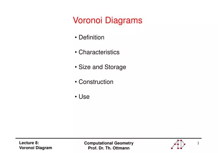
Definition • Characteristics • Size and Storage • Construction • Use Voronoi Diagrams Computational Geometry Prof. Dr. Th. Ottmann

The Voronoi Diagram Computational Geometry Prof. Dr. Th. Ottmann

Voronoi Regions Eucledian distance : dist(p,q) := Let P :={ p1, p2, ...,pn } be a set of n distinct points in a plane.We define the voronoi diagram of P as the subdivision of the planeinto n cells, with the property that a point q lies in the cell correspon-ding to a site pi iff dist(q, pi ) < dist(q, pj ) for each pj P with j  i. We denote the Voronoi diagram of P by Vor(P).The cell that corresponds to a site piis denotd by V(pi ), called thevoronoi cell of pi. Computational Geometry Prof. Dr. Th. Ottmann

Example V(pi) = 1 j  n, j  i h(pi, pj) q1 q2 p q4 q3 Computational Geometry Prof. Dr. Th. Ottmann

Computing the Voronoi Diagram Input: A set of points (sites) Output: A partitioning of the plane into regions of equal nearest neighbors Computational Geometry Prof. Dr. Th. Ottmann

Animations of the Voronoi diagram Java Applet zur Animation von Voronoi Diagrammen, Entwickelt von R. Klein u.a., FU Hagen pi V(pi) Computational Geometry Prof. Dr. Th. Ottmann

Characteristics of Voronoi Diagrams (1) Voronoi regions (cells) are bounded by line segments. Special case : Collinear points Theorem : Let P be a set of n points (sites) in the plane.If all the sites are collinear, then Vor(P) consist of n-1 parallel lines and n cells. Otherwise, Vor(P) is a connected graph and its edges are either line segments or half-lines. If pi, pjare notcollinearwithpk, thenh(pi, pj ) and h(pj, pk ) can not be parallel! e pk pi pj h(pj,pk) h(pi,pj) Computational Geometry Prof. Dr. Th. Ottmann

Vor(P) is Connected Claim: Vor(P) is connected Proof by contradiction: If Vor(P) is not connected then there would be a Voronoicell V(Pi ) splitting the plane into two halfes. Because Voronoi cells are convex, V(Pi ) would consist of a strip bounded by two parallel full lines, but we know that edges of Voronoi diagram cannot be full lines, hence a contradiction. Computational Geometry Prof. Dr. Th. Ottmann

Other Characteristics (Assumption: No 4 points are on the circle) (2) Each vertex (corner) of VD(P) has degree 3 (3) The circle through the three points defining a Vertex of the Voronoi diagram does not contain any further point Computational Geometry Prof. Dr. Th. Ottmann

(4) Each nearest neighbor of one point defines an edge of the Voronoi region of the point. (5) The Voronoi region of a point is unbounded iff the point lies exactly on the convex hull of the point set. Computational Geometry Prof. Dr. Th. Ottmann

Size and Storage Size of the Voronoi Diagram: V(p) can have O(n) vertices! Computational Geometry Prof. Dr. Th. Ottmann

Size of the Voronoi Diagram Theorem: The number of vertices in the Voronoi diagram of a set of n points in the plane is at most 2n-5 and the number of edges is at most 3n-6. • Proof:1. Connect all Half-lines with fictitious point 2. Apply Euler`s formula:v – e + f = 2 • For VD(P) +  :v = number of vertices of VD(P) + 1e = number of edges of VD(P)f = number of sites of VD(P) = n • Each edge in VD(P) +  has exactly two vertices and each vertexof VD(P) + has at least a degree of 3: • sum of the degrees of all vertices ofVor(P) + = 2·( # edges of VD(P) )  3· (# vertices of VD(P) + 1) Computational Geometry Prof. Dr. Th. Ottmann

Proof(Continued) Number of vertices ofVD(P) = vp Number of edges of VD(P) = ep We can apply:(vp + 1) – ep + n = 2 2 ep  3 (vp + 1) 2 ep  3 ( 2 + ep - n) = 6 + 3ep – 3n 3n – 6  ep Computational Geometry Prof. Dr. Th. Ottmann

Example Computational Geometry Prof. Dr. Th. Ottmann

Storage of Voronoi-Diagrams Three Records: vertex { Coordinates Incident edge };face { OuterComponent InnerComponents };halfedge { Origin Twin IncidentFace Next Prev }; 4 3 2 5 3 1 4 6 1 2 5 e.g. : Vertices 1 = {(1,2) | 12}Sites 1 = {15 | [] }Edges 54 = { 4 | 45 | 1 | 43 | 15 } Computational Geometry Prof. Dr. Th. Ottmann

Computing the Voronoi Diagram Input: A set of points (sites) Output: A partitioning of the plane into regions of equal nearest neighbors. Computational Geometry Prof. Dr. Th. Ottmann

Divide and Conquer(Divide) Input: A set of points (sites) Output: A partitioning of the plane into regions of equal nearest neighbors. Divide: Divide the point set into two halves Computational Geometry Prof. Dr. Th. Ottmann

Divide and Conquer (Conquer) Conquer: Recursively compute the Voronoi diagrams for the smaller point sets Abort condition: Voronoi diagram of a single point is theentire plane. Computational Geometry Prof. Dr. Th. Ottmann

Divide and Conquer (Merge) Merge the diagrams by a (monoton) sequence of edges) Computational Geometry Prof. Dr. Th. Ottmann

The Result The finished Voronoi Diagram Running time: With n given points is O(n log n) Computational Geometry Prof. Dr. Th. Ottmann

Geometrical Divide and Conquer A D B E C Problem: Determine all intersecting pairs of segments S A A D B D B E C E C S1 S2 Computational Geometry Prof. Dr. Th. Ottmann

DAC - Construction of the Voronoi diagram Divide:Divide P by a vertical dividing line T into 2 equal size subsets say P1 and P2. If |P|= 1completed. Conquer:Compute VD(P1 ) and VD(P2 ) recursively. Merge: Compute the edge sequence K separating P1 and P2Cut VD(P1) and VD(P2 ) by means of K starting from VD(P1 ) and VD(P2 ) and K P2 P1 T Theorem:If K can be computed in time O(n), then the running time of the D&C-algorithm is T(n) = O(n logn) Proof :T(n) = 2 T(n/2) + O(n),T(1) =O(1) Computational Geometry Prof. Dr. Th. Ottmann

Computation of K First edge in K P1 P2 Last edge in K 4 tangentialpointsP1 P2Observation:K is y - monotonous Incremental (sweep line) construction(p1 in P1 and p2 in P2perpendicular with m, Sweep l) Determines intersections1 of m with Vor(p1) below l Determines intersection s2 of m with Vor(p2) belowl Extend K by line segment l si Set l = si Compute new K defining pair p1,p2 Theorem: Running time O(n) Proof:Vor(pi) are convex, therefore each one‘sforward - edge are only visitedonce. Computational Geometry Prof. Dr. Th. Ottmann

Example Computational Geometry Prof. Dr. Th. Ottmann

Fortune´s Algorithm Observations: Intersection of the parabolas define edges New "telephones" ( ) define new parabolas Parabola intersection disappear, if C(P, q) has 3 points Beach - line Sweep - line Computational Geometry Prof. Dr. Th. Ottmann

Applications 1(Static Point Set) Closest pair of points: Go through edge list for VD(P) and determine minimum All next neighbors : Go through edge list for VD(P) for all points and get next neighbors in each case • Minimum Spanning tree (after Kruskal) • Each point p from P defines1-element set of • More than a set of T exists • 2.1) find p,p´ with p in T and p´ not in Twith d(p, p´)minimum. • 2.2) connect T and p´ contained in T´ (union) Theorem: The MST can be computed in time O(n log n) Computational Geometry Prof. Dr. Th. Ottmann

Applications (dynamic object set) a A b c Search for next neighbor : Idea: Hierarchical subdivision of VD(P) Step 1 :Triangulation of final Voronoi regions Step 2 : Summary of triangles and structure of a search tree Rule of Kirkpatrick: Remove in each case points withdegree < 12, its neighbor is already far. A a c b Theorem:Using the rule of Kirkpatrick a search tree of logarithmic depth develops. Computational Geometry Prof. Dr. Th. Ottmann

Voronoi Diagrams