Towards Improving Coupled Climate Model Using EnKF Parameter Optimization

1. Towards Improving Coupled Climate Model Using EnKF Parameter Optimization Zhengyu Liu1, Shaoqing Zhang2, Yun Liu1 R. Jacob3, Xinrong Wu4, Xuefeng Zhang4, Feiyu Lu1 1. Univ. Wisconsin-Madison 2. GFDL/NOAA, USA 3. ANL/DOE 4. NMDIS/SOA, China

2. Motivation: Coupled Model Biases SST (shading), Rainfall (contour) Prep Latitude Lin, 2007, JC

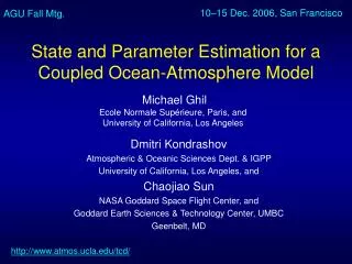
3. Objective Improve a complex climate model directly in the coupled mode? (after the tuning of each component model) Model biases Structure biases Parameter biases Parameter Estimation using Data Assimilation: 4D Var: adjoint in CGCM EnKF: forward modeling, practical for a complex system

4. EnKF Parameter Optimization Anderson, J., 2001: Lorenz Model: Variable Augmentation Meso-scale weather model Objective: improve forecasting error, Approach: time-marching EnKF on synoptic obs (Anderson, 2001) Aksoy et al., 2006a (perfect model) Aksoy et al, 2006b (perfect model) Tong and Xue, 2007 (perfect model) Hu et al., 2010 (real data) ……. Climate model Objective: reduce climatology bias for projection Approach: Iterative EnKF on climatological obs (Annan et al., 2004) Annan et al., 2005: AGCM (reanalysis atmosphere) Edwards and March, 2005: OGCM (perfect model, ocean obs) Ridgewell et al., 2007: Marine BGC model (real data, ocean obs) and prediction

5. EnKF Parameter Optimization for Coupled Models Potential Issues • Different time scales: fast processes, slow processes, coupled processes • Biases in climatology, climate variability, “climate noise” e.g: tropical bias, ENSO, NAO,.. atmos. synoptics • Biases in single component (before coupling) vs. coupled system • Atmosphere obs + Ocean obs + (other system component obs) • Great spatial variation: low vs high lat? ocean vs land? …. …..

6. EnKF Parameter Optimization for Coupled Models Outline • A conceptual coupled model study (perfect model) Zhang S., Liu, Z., A. Rosati and T. Delworthy, 2012. A study of enhancive parameter correction with coupled data assimilation for climate simulation and prediction using a simple coupled model. Tellus, A first try! • A CGCM study (perfect model) Liu Y., Z. Liu, S. Zhang, X. Rong, R. Jacob, S. Wu and F. Lu, 2014: Ensemble-based parameter estimation in a coupled GCM using the adaptive spatial average method. J. Climate (in press) First Success in CGCM! • A intermediate coupled model study (“biased physics”) Zhang X., S. Zhang, Z. Liu, X. Wu and G. Han, 2014: Parameter optimization in an intermediate coupled climate model with biased physics. J. Climate (in rev) Further challenges… All use EAKF (Anderson, J., 2001)

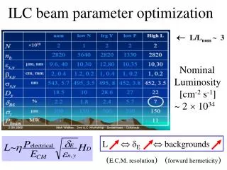
7. A Conceptual Model Study (“Perfect Model”) Obs Frq: different in A (1 day) and O (4 day) N=20 Initial para error ~10% Fixed low threshold of para ensemble spread (as in Askoy et al. 2006) Correlation cut-off Atmos Ocean (Om=10) Spin-up Step 1: State estimation to quasi-equilibrium Step 2: Simultaneous state-para estimation Zhang S. et al., 2011, Tellus

8. Multi-parameter Estimation Zhang S. et al., 2011, Tellus

9. A CGCM Study (“Perfect Model”) Fast Ocean Atmosphere Model (FOAM) (Jacob, 2007) Atmosphere: CCM2 R15 +CCM3 Physics Ocean: POP-like 2.4ox1.2ox24-levels Obs. Err = 10% Std(CTRL) SST Obs: 1 monthly (gridded) Atmosphere Obs: T, U, V, 12 hrly (gridded) N=30 members Ocean/Atmosphere coupling covariance not used Localization: atmos: 1000 km, ocn:500 km Parameters: Solar Penetration Depth (SPD) + Other parameters Liu Y., PH.D thesis Liu Y. et al., 2014a,b, J. Clim

10. Parameter Sensitivity a) D SST: ann. SPD 20m - 17m a) SST: ann. climatology sensitivity Climatology sensitivity b) <SST, SST> 1 month sensitivity Ensemble spread: June c) <SST, SST> 1 month sensitivity, Ensemble spread Dec Liu Y. et al., 2014, J. Clim a) SST: ann. climatology sensitivity a) SST: ann. climatology sensitivity a) SST: ann. climatology sensitivity b) SST: 1 month sensitivity (June) b) SST: 1 month sensitivity (June) b) SST: 1 month sensitivity (June) c) SST: 1 month sensitivity (Dec) c) SST: 1 month sensitivity (Dec) c) SST: 1 month sensitivity (Dec)

11. Estimation of SPD Year Assimilation of monthly SST obs only Liu Y. et al., 2014, J. Clim

12. Adaptive Spatial Average Scheme (ASA) For a global uniform parameter Spatial updating (localization): GPO (Wu et al. 2012) SA(Spatial Average): Askoy et al., 2006 ASA (Adaptive Spatial Average): Liu Y. et al., 2014 Liu Y. et al., 2014, J. Clim

13. Spatial Variation of Parameter Sensitivity a) D SST: ann. SPD 20m - 17m a) SST: ann. climatology sensitivity Climatology sensitivity b) <SST, SST> 1 month sensitivity Ensemble spread: June c) <SST, SST> 1 month sensitivity, Ensemble spread Dec Liu Y. et al., 2014, J. Clim a) SST: ann. climatology sensitivity a) SST: ann. climatology sensitivity a) SST: ann. climatology sensitivity b) SST: 1 month sensitivity (June) b) SST: 1 month sensitivity (June) b) SST: 1 month sensitivity (June) c) SST: 1 month sensitivity (Dec) c) SST: 1 month sensitivity (Dec) c) SST: 1 month sensitivity (Dec)

14. ASA: Quality of Estimation and Ensemble Spread Obs = truth Obs = truth + error rmse(SPD) σ(SPD) ASA (Adaptive Spatial Average): A good estimate ~ small posterior ensemble spread σ(β) β=SPD x=SST rmse(SPD) rmse(SPD) σ(SPD) σ(SPD) SPD SPD Liu Y. et al., 2014, J. Clim % average grids % average grids

15. Summary • Preliminary results encouraging • Parameter optimization seems feasible for CGCMs, but • Real world parameter optimization most challenging! Different time scales…? Spatial and temporal (stochastic) variation ? Flux adjustment? Physical mechanism ? (breeding mode?) Earth system model?