Download
1 / 58
950 likes | 4.09k Vues
Chapter 6: Distribution and Network Models. Instructor: Dr. Neha Mittal. Introduction. A special class of linear programming problems is called Network Flow problems. Five different problems are considered: Transportation Problems Assignment Problems Transshipment Problems

E N D
Chapter 6: Distribution and Network Models Instructor: Dr. Neha Mittal
Introduction • A special class of linear programming problems is called Network Flow problems. Five different problems are considered: • Transportation Problems • Assignment Problems • Transshipment Problems • Shortest-Route Problems • Maximal Flow Problems
Transportation, Assignment, and Transshipment Problems • They are all network models, represented by a • set of nodes, • a set of arcs, • and functions (e.g. costs, supplies, demands, etc.) associated with the arcs and/or nodes.
In this chapter: • Transportation & Assignment Problems • Network Representation • General LP Formulation • Solution with QM Software • Transshipment Problem • Network Representation • General LP Formulation
Transportation Problem • The transportation problem seeks to minimize the total shipping costs of transporting goods from m origins (each with a supply si) to n destinations (each with a demand dj), when the unit shipping cost from an origin, i, to a destination, j, is cij. • The network representation for a transportation problem with two sources and three destinations is given on the next slide.
Transportation Problem • Network Representation 1 d1 c11 1 c12 s1 c13 2 d2 c21 c22 2 s2 c23 3 d3 Sources Destinations
Transportation Problem • Linear Programming Formulation Using the notation: xij = number of units shipped from origin i to destination j cij= cost per unit of shipping from origin i to destination j si = supply or capacity in units at origin i dj = demand in units at destination j
= Transportation Problem • Linear Programming Formulation (continued) xij> 0 for all i and j
LP Formulation Special Cases • The objective is maximizing profit or revenue: • Minimum shipping guarantee from i to j: xij>Lij • Maximum route capacity from i to j: xij<Lij • Unacceptable route: Remove the corresponding decision variable. Solve as a maximization problem.
Transportation Problem: Example #1 Acme Acme Block Company has orders for 80 tons of concrete blocks at three suburban locations as follows: Northwood -- 25 tons, Westwood -- 45 tons, and Eastwood -- 10 tons. Acme has two plants, each of which can produce 50 tons per week. Delivery cost per ton from each plant to each suburban location is shown on the next slide. How should end of week shipments be made to fill the above orders?
Delivery Cost Per Ton NorthwoodWestwoodEastwood Plant 1 24 30 40 Plant 2 30 40 42
Network Representation Demand Unit Costs 1 North Supply 25 24 1 Plant 1 50 30 40 2West 45 30 2 Plant 2 40 50 42 3 East 10 Origins Destinations
Shipment Cost Minimization / LP Formulation Decision variables: xij = Amount shipped for i = 1-2 and j = 1-3 Min Z = 24x11 + 30x12 + 40x13 + 30x21 + 40x22 + 42x23 s.t. x11 + x12 + x13 < 50 (Plant 1 capacity) x21 + x22 + x23 < 50 (Plant 2 capacity) x11 + x21 = 25 (Northwood demand) x12 + x22 = 45 (Westwood demand) x13 + x23 = 10 (Eastwood demand) xij > 0 for i = 1-2 origins, j = 1-3 destinations
Optimal Solution (Minimizing Cost) FromToAmountCost Plant 1 Northwood 5 120 Plant 1 Westwood 45 1,350 Plant 2 Northwood 20 600 Plant 2 Eastwood 10 420 Total Cost = $2,490 Notes: Supply from Plant 2 is not fully utilized (excess shown in ‘Dummy’ column in QM). Also, nothing is shipped from Plant 1 to Eastwood or from Plant 2 to Westwood. The unit cost for that route must decrease more than the marginal cost (shown in QM) in order to be utilized.
QM Output (using “Transportation” Module) Transportation Shipments Window 1) Which plant has excess supply? How much? 2) What the unit cost of shipments from Plant 1 to Eastwood would have to be in order for that route to be utilized (original cost = $40) Marginal Costs Window
Transportation Problem: Example #2 The Navy has 9,000 pounds of material in Albany, Georgia that it wishes to ship to three destinations: San Diego, Norfolk, and Pensacola. They require 4,000, 2,500, and 2,500 pounds, respectively. There are three different carriers and government regulations require equal distribution of shipping among the three carriers.
The shipping costs per pound for truck, railroad, and airplane transit are shown below. Formulate and solve a linear program to determine the shipping arrangements (mode, destination, and quantity) that will minimize the total shipping cost. Destination Mode San Diego Norfolk Pensacola Truck $12 $ 6 $ 5 Railroad 20 11 9 Airplane 30 26 28
Decision Variables We want to determine the pounds of material, xij , to be shipped by mode i to destination j. The following table summarizes the decision variables: San Diego Norfolk Pensacola Truckx11x12x13 Railroad x21x22x23 Airplane x31x32x33
Objective Function Minimize the total shipping cost. Min: (shipping cost per pound for each mode per destination pairing) x (number of pounds shipped by mode per destination pairing). Min: 12x11 + 6x12 + 5x13 + 20x21 + 11x22 + 9x23 + 30x31 + 26x32 + 28x33
Constraints Equal use of transportation modes: (1) x11 + x12 + x13 = 3000 (2) x21 + x22 + x23 = 3000 (3) x31 + x32 + x33 = 3000 Destination material requirements: (4) x11 + x21 + x31 = 4000 (5) x12 + x22 + x32 = 2500 (6) x13 + x23 + x33 = 2500 Non-negativity of variables: xij> 0, i = 1,2,3 and j = 1,2,3
Solution Summary • San Diego will receive 1000 lbs. by truck and 3000 lbs. by airplane. • Norfolk will receive 2000 lbs. by truck and 500 lbs. by railroad. • Pensacola will receive 2500 lbs. by railroad. • The total shipping cost will be $142,000.
Practice Problem Powerco has three electric power plants that supply the electric needs of four cities. The associated supply of each plant and demand of each city is given in the table. The cost of sending 1 million kwh of electricity from a plant to a city depends on the distance the electricity must travel. Determine how much energy should be supplied to the city by which plant?
Costs to Haul from each site to each mill (round-trip costs) are given below:
Assignment Problem • An assignment problem seeks to minimize the total cost assignment of i workers to j jobs, given that the cost of worker i performing job j is cij. • It assumes all workers are assigned and each job is performed. • An assignment problem is a special case of a transportation problem in which all supplies and all demands are equal to 1; hence assignment problems may be solved as linear programs. • The network representation of an assignment problem with three workers and three jobs is shown on the next slide.
Network Representation c11 1 1 c12 c13 Agents Tasks c21 c22 2 2 c23 c31 c32 3 3 c33
Linear Programming Formulation Using the notation: xij = 1 if agent i is assigned to task j 0 otherwise cij= cost of assigning agent i to task j
Linear Programming Formulation (continued) xij> 0 for all i and j
LP Formulation Special Cases • Number of agents exceeds the number of tasks: • Number of tasks exceeds the number of agents: • Add enough dummy agents to equalize the number of • agents and the number of tasks. The objective function • coefficients for these new variable would be zero. Extra agents simply remain unassigned.
LP Formulation Special Cases (continued) • The assignment alternatives are evaluated in terms of revenue or profit: • Solve as a maximization problem. • An assignment is unacceptable: Remove the corresponding decision variable. • An agent is permitted to work t tasks:
Practice Problem An electrical contractor pays his subcontractors a fixed fee plus mileage for work performed. On a given day the contractor is faced with three electrical jobs associated with various projects. Given below are the distances between the subcontractors and the projects. Projects SubcontractorABC Westside 50 36 16 Federated 28 30 18 Goliath 35 32 20 Universal 25 25 14 How should the contractors be assigned to minimize total mileage costs?
Network Representation 50 West. A 36 16 Subcontractors Projects 28 30 Fed. B 18 32 35 Gol. C 20 25 25 Univ. 14
Linear Programming Formulation Min 50x11+36x12+16x13+28x21+30x22+18x23 +35x31+32x32+20x33+25x41+25x42+14x43 s.t. x11+x12+x13 < 1 x21+x22+x23 < 1 x31+x32+x33 < 1 x41+x42+x43 < 1 x11+x21+x31+x41 = 1 x12+x22+x32+x42 = 1 x13+x23+x33+x43 = 1 xij = 0 or 1 for all i and j Agents Tasks Note: If #agents = #tasks, first 4 constraints would have been “= 1” instead of “< 1”
QM Select the “Assignment” Module “Jobs” are the same as Projects “Machines” are whatever/whoever is performing the Jobs If assignments are being evaluated for Cost Select Minimize Revenue/Profit Select Maximize
Problem Machineco has four machine and four jobs to be completed. Each machine must be assigned to complete one job. The time required to set up each machine for completing each job is shown below. Formulate the problem to minimize the total setup time needed to complete the four jobs. Job1 Job2 Job3 Job4 Machine1 14 5 8 7 Machine2 2 12 6 5 Machine3 7 8 3 9 Machine4 2 4 6 10
Problem Three professors must be assigned to teach six sections of Management Science. Each professor can teach up to two sections. Each has ranked the six time periods during which MS is taught. Higher the ranking, higher is the desirability of the professor to teach at that time. Determine an assignment of professors to sections. 9AM 10 11 1 2 3PM Professor1 8 7 6 5 7 6 Professor2 9 9 8 8 4 4 Professor3 7 6 9 6 9 9
Transshipment Problem • Transshipment problems are transportation problems in which a shipment may move through intermediate nodes (transshipment nodes) before reaching a particular destination node. • The network representation for a transshipment problem with two sources, three intermediate nodes, and two destinations is shown on the next slide.
Network Representation c36 3 c13 c37 1 6 s1 d1 c14 c46 c15 4 Demand c47 Supply c23 c56 c24 7 2 d2 s2 c25 5 c57 Destinations Sources Intermediate Nodes
Linear Programming Formulation Using the notation: xij = number of units shipped from node i to node j cij = cost per unit of shipping from node i to node j si= supply at origin node i dj= demand at destination node j
Linear Programming Formulation (continued) xij> 0 for all i and j
Special Cases • Total supply not equal to total demand • Maximization objective function • Route capacities or route minimums • Unacceptable routes • The LP model modifications required here are • identical to those required for the special cases in • the transportation problem.
Transshipment Problem: Example The Northside and Southside facilities of Zeron Industries supply three firms (Zrox, Hewes, Rockrite) with customized shelving for its offices. They both order shelving from the same two manufacturers, Arnold Manufacturers and Supershelf, Inc. Currently weekly demands by the users are 50 for Zrox, 60 for Hewes, and 40 for Rockrite. Both Arnold and Supershelf can supply at most 75 units to its customers. Additional data is shown on the next slide.
Because of long standing contracts based on past orders, unit costs from the manufacturers to the suppliers are: Zeron NZeron S Arnold 5 8 Supershelf 7 4 The costs to install the shelving at the various locations are: ZroxHewesRockrite Zeron N 1 5 8 Zeron S 3 4 4